Identify mangrove forests using satellite image features using Amazon SageMaker Studio and Amazon SageMaker Autopilot – Part 1

{"value":"The increasing ubiquity of satellite data over the last two decades is helping scientists observe and monitor the health of our constantly changing planet. By tracking specific regions of the Earth’s surface, scientists can observe how regions like forests, water bodies, or glaciers change over time. One such region of interest for geologists is mangrove forests. These forests are essential to the overall health of the planet and are one of the many areas across the world that are impacted by human activities. In this post, we show how to get access to satellite imagery data containing mangrove forests and how to visually interact with the data in ++[Amazon SageMaker Studio](https://docs.aws.amazon.com/sagemaker/latest/dg/studio.html)++. In ++[Part 2](https://aws.amazon.com/blogs/machine-learning/part-2-identify-mangrove-forests-using-satellite-image-features-using-amazon-sagemaker-studio-and-amazon-sagemaker-autopilot/)++ of this series, we show how to train a machine learning (ML) model using ++[Amazon SageMaker Autopilot](https://aws.amazon.com/sagemaker/autopilot/)++ to identify those forests from a satellite image.\n\n### **Overview of solution**\n\nA large number of satellites orbit the Earth, scanning its surface on a regular basis. Typical examples of such satellites are Landsat, Sentinel, CBERS, and MODIS, to name a few. You can access both recent and historical data captured by these satellites at no cost from multiple providers like [USGS EarthExplorer](https://earthexplorer.usgs.gov/), [Land Viewer](https://eos.com/products/landviewer/), or [Copernicus Open Access Hub](https://scihub.copernicus.eu/). Although they provide an excellent service to the scientific community by making their data freely available, it takes a significant amount of effort to gain familiarity with the interfaces of the respective providers. Additionally, such data from satellites is made available in different formats and may not comply with the standard Geographical Information Systems (GIS) data formatting. All of these challenges make it extremely difficult for newcomers to GIS to prepare a suitable dataset for ML model training.\n\nPlatforms like [Google Earth Engine](https://earthengine.google.com/) (GEE) and [Earth on AWS](https://aws.amazon.com/earth/) make a wide variety of satellite imagery data available in a single portal that eases searching for the right dataset and standardizes the ETL (extract, transform, and load) component of the ML workflow in a convenient, beginner-friendly manner. GEE additionally provides a coding platform where you can programmatically explore the dataset and build a model in JavaScript. The Python API for GEE lacks the maturity of its JavaScript counterpart; however, that gap is sufficiently bridged by the open-sourced project geemap.\n\nIn this series of posts, we present a complete end-to-end example of building an ML model in the GIS space to detect mangrove forests from satellite images. Our goal is to provide a template solution that ML engineers and data scientists can use to explore and interact with the satellite imagery, make the data available in the right format for building a classifier, and have the option to validate model predictions visually. Specifically, we walk through the following:\n\n- How to download satellite imagery data to a Studio environment\n- How to interact with satellite data and perform exploratory data analysis in a Studio notebook\n- How to automate training an ML model in Autopilot\n\n### **Build the environment**\n\nThe solution presented in this post is built in a Studio environment. To configure the environment, complete the following steps:\n\n1. Add a new SageMaker domain user and launch the Studio app. (For instructions, refer to [Get Started](https://docs.aws.amazon.com/sagemaker/latest/dg/notebooks-get-started.html).)\n2. Open a new Studio notebook by choosing the plus sign under **Notebook and compute resources** (make sure to choose the Data Science SageMaker image).\n\n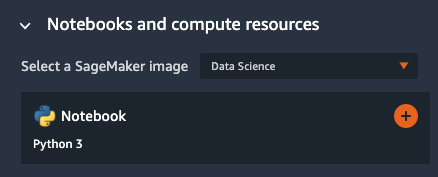\n\n3. Clone the [mangrove-landcover-classification](https://github.com/aws-samples/mangrove-landcover-classification) Git repository, which contains all the code used for this post. (For instructions, refer to [Clone a Git Repository in SageMaker Studio](https://docs.aws.amazon.com/sagemaker/latest/dg/studio-tasks-git.html)).\n4. Open the \nnotebook ```notebooks/explore_mangrove_data.ipynb```.\n5. Run the first notebook cell to pip install all the required dependencies listed in the requirements.txt file in the root folder.\n6. Open a new Launcher tab and open a system terminal found in the Utilities and files section.\n\n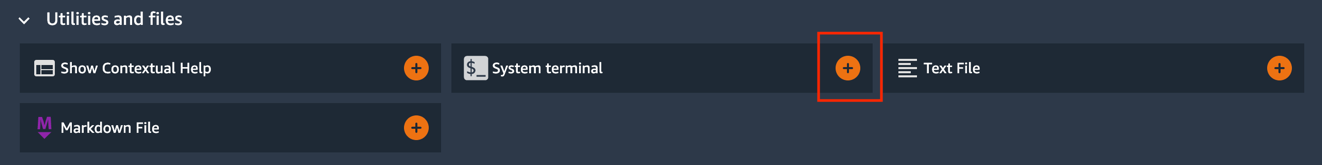\n\n7. Install the Earth Engine API:\n\n```\\npip install earthengine-api\\n```\n\n8. Authenticate Earth Engine:\n\n```\\nearthengine authenticate\\n```\n\n\n\n9. Follow the Earth Engine link in the output and [sign up](https://earthengine.google.com/signup/) as a developer so that you can access GIS data from a notebook.\n\n### **Mangrove dataset**\n\nThe [Global Mangrove Forest Distribution](https://developers.google.com/earth-engine/datasets/catalog/LANDSAT_MANGROVE_FORESTS) (GMFD) is one of the most cited datasets used by researchers in the area. The dataset, which contains labeled mangrove regions at a 30-meter resolution from around the world, is curated from more than 1,000 [Landsat](https://landsat.gsfc.nasa.gov/) images obtained from the [USGS EROS](https://www.usgs.gov/centers/eros) Center. One of the disadvantages of using the dataset is that it was compiled in 2000. In the absence of a newer dataset that is as comprehensive as the GMFD, we decided to use it because it serves the purpose of demonstrating an ML workload in the GIS space.\n\nGiven the visual nature of GIS data, it’s critical for ML practitioners to be able to interact with satellite images in an interactive manner with full map functionalities. Although GEE provides this functionality through a [browser interface](https://code.earthengine.google.com/), it’s only available in JavaScript. Fortunately, the open-sourced project geemap aids data scientists by providing those functionalities in Python.\n\nGo back to the ```explore_mangrove_data.ipynb``` notebook you opened earlier and follow the remaining cells to understand how to use simple interactive maps in the notebook.\n\n1. Start by importing Earth Engine and initializing it:\n\n```\\nimport ee\\nimport geemap.eefolium as geemap\\nee.Initialize()\\n```\n\n2. Now import the satellite image collection from the database:\n\n```\\nmangrove_images_landsat = ee.ImageCollection('LANDSAT/MANGROVE_FORESTS')\\n```\n\n3. Extract the collection, which contains just one set:\n\n```\\nmangrove_images_landsat = mangrove_images_landsat.first()\\n```\n\n4. To visualize the data on a map, you first need to instantiate a map through geemap:\n\n```\\nmangrove_map = geemap.Map()\\n```\n\n5. Next, define some parameters that make it easy to visualize the data on a world map:\n\n```\\nmangrovesVis = {\\n min: 0,\\n max: 1.0,\\n 'palette': ['d40115'],\\n }\\n```\n\n6. Now add the data as a layer on the map instantiated earlier with the visualization parameters:\n\n```\\nmangrove_map.addLayer(mangrove_images_landsat, mangrovesVis, 'Mangroves')\\n```\n\nYou can add as many layers as you want to the map and then interactively turn them on or off for a cleaner view when necessary. Because mangrove forests aren’t everywhere on the earth, it makes sense to center the map to a coastal region with known mangrove forests and then render the map on the notebook as follows:\n\n```\\nmangrove_map.setCenter(-81, 25, 9)\\nmangrove_map\\n```\n\nThe latitude and longitude chosen here, 25 degrees north and 81 degrees west, respectively, correspond to the gulf coast of Florida, US. The map is rendered at a zoom level of 9, where a higher number provides a more closeup view.\n\n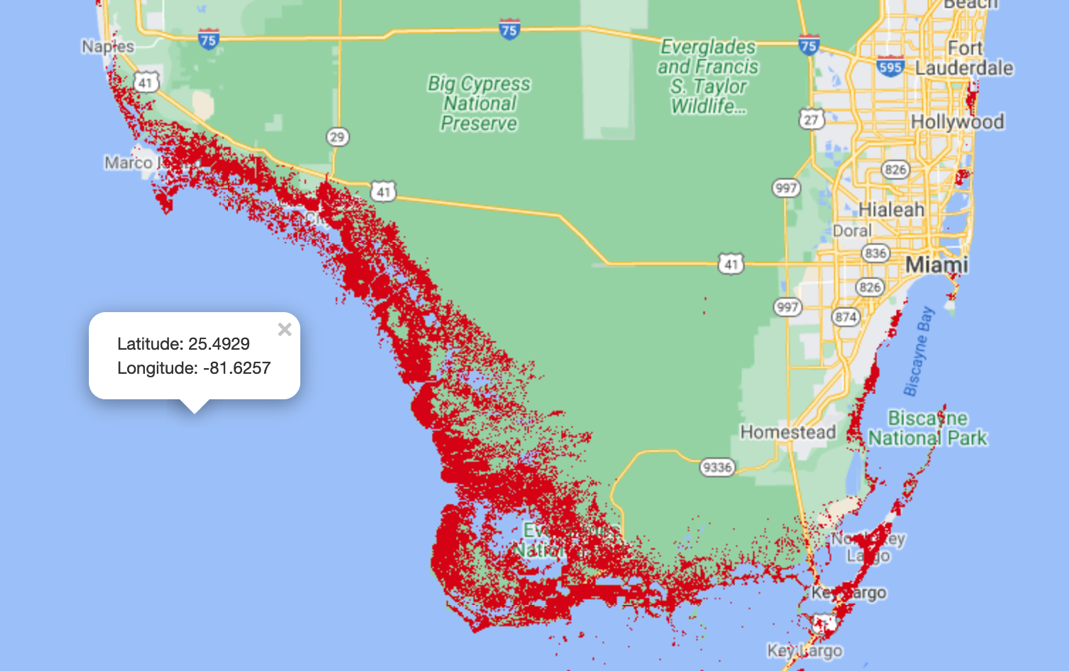\n\nYou can obtain some useful information about the dataset by accessing the associated metadata as follows:\n\n```\\ngeemap.image_props(mangrove_images_landsat).getInfo()\\n```\n\nYou get the following output:\n\n```\\n{'IMAGE_DATE': '2000-01-01',\\n 'NOMINAL_SCALE': 30.359861978395436,\\n 'system:asset_size': '41.133541 MB',\\n 'system:band_names': ['1'],\\n 'system:id': 'LANDSAT/MANGROVE_FORESTS/2000',\\n 'system:index': '2000',\\n 'system:time_end': '2001-01-01 00:00:00',\\n 'system:time_start': '2000-01-01 00:00:00',\\n 'system:version': 1506796895089836\\n}\\n```\n\nMost of the fields in the metadata are self-explanatory, except for the band names. The next section discusses this field in more detail.\n\n### **Landsat dataset**\n\nThe following image is a satellite image of an area at the border of French Guiana and Suriname, where mangrove forests are common. The left image shows a raw satellite image of the region; the image on the right depicts the GMFD data superimposed on it. Pixels representing mangroves are shown in red. It’s quite evident from the side-by-side comparison that there is no straightforward visual cue in either structure or color in the underlying satellite image that distinguishes mangroves from the surrounding region. In the absence of any such distinguishing pattern in the images, it poses a considerable challenge even for state-of-the-art deep learning-based classifiers to identify mangroves accurately. Fortunately, satellite images are captured at a range of wavelengths on the electromagnetic spectrum, part of which falls outside the visible range. Additionally, they also contain important measurements like surface reflectance. Therefore, researchers in the field have traditionally relied upon these measurements to build ML classifiers.\n\n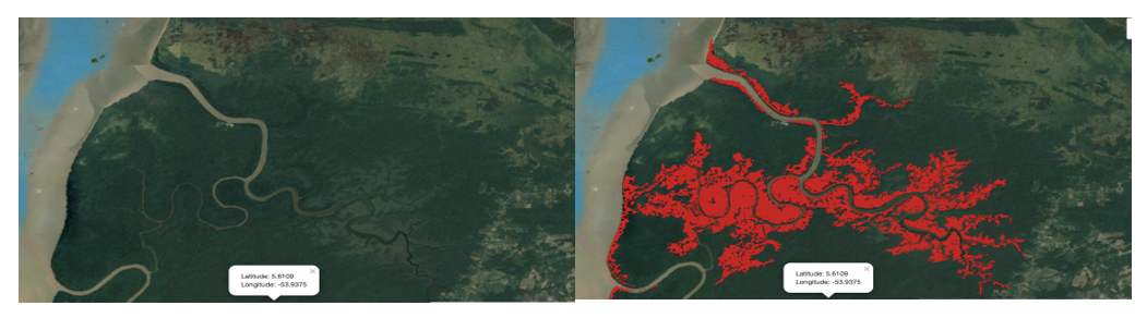\n\nUnfortunately, apart from marking whether or not an individual pixel represents mangroves, the GMFD dataset doesn’t provide any additional information. However, other datasets can provide a host of features for every pixel that can be utilized to train a classifier. In this post, you use the [USGS Landsat 8 dataset](https://www.usgs.gov/core-science-systems/nli/landsat/landsat-surface-reflectance?qt-science_support_page_related_con=0#qt-science_support_page_related_con) for that purpose. The [Landsat 8](https://www.usgs.gov/core-science-systems/nli/landsat/landsat-8?qt-science_support_page_related_con=0) satellite was launched in 2013 and orbits the Earth every 99 minutes at an altitude of 705 km, capturing images covering a 185 km x 180 km patch on the Earth’s surface. It captures nine spectral bands, or portions of the electromagnetic spectrum sensed by a satellite, ranging from ultra blue to shortwave infrared. Therefore, the images available in the Landsat dataset are a collection of image patches containing multiple bands, with each patch time stamped by the date of collection.\n\nTo get a sample image from the Landsat dataset, you need to define a point of interest:\n\n```\\npoint = ee.Geometry.Point([<longitude>, <latitude>])\\n```\n\nThen you filter the image collection by the point of interest, a date range, and optionally by the bands of interest. Because the images collected by the satellites are often obscured by cloud cover, it’s absolutely necessary to extract images with the minimum amount of cloud cover. Fortunately, the Landsat dataset already comes with a cloud detector. This streamlines the process of accessing all available images over several months, sorting them by amount of cloud cover, and picking the one with minimum cloud cover. For example, you can perform the entire process of extracting a Landsat image patch from the northern coast of the continent of South America in a few lines of code:\n\n```\\npoint = ee.Geometry.Point([-53.94, 5.61])\\nimage_patch = ee.ImageCollection('LANDSAT/LC08/C01/T1_SR') \\\\\\n .filterBounds(point) \\\\\\n .filterDate('2016-01-01', '2016-12-31') \\\\\\n .select('B[1-7]') \\\\\\n .sort('CLOUD_COVER') \\\\\\n .first()\\n```\n\nWhen specifying a region using a point of interest, that region doesn’t necessarily have to be centered on that point. The extracted image patch simply contains the point somewhere within it.\n\nFinally, you can plot the image patch over a map by specifying proper plotting parameters based on a few of the chosen bands:\n\n```\\nvis_params = {\\n \\t\\t\\t'min': 0,\\n'max': 3000,\\n'bands': ['B5', 'B4', 'B3']\\n }\\nlandsat = geemap.Map()\\nlandsat.centerObject(point, 8)\\nlandsat.addLayer(image_patch, vis_params, \\"Landsat-8\\")\\nlandsat\\n```\n\nThe following is a sample image patch collected by Landsat 8 showing in false color the Suriname-French Guiana border region. The mangrove regions are too tiny to be visible at the scale of the image.\n\n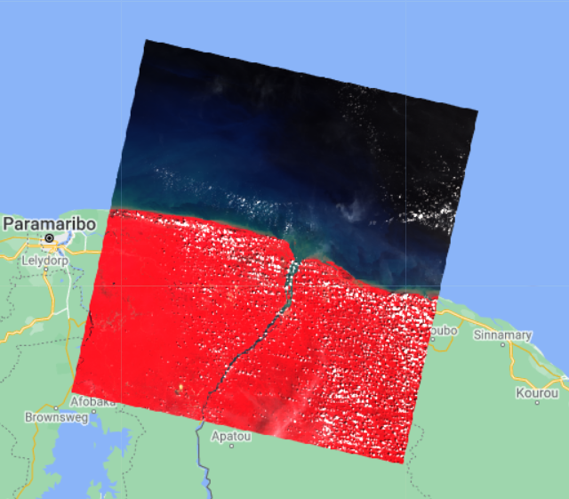\n\nAs usual, there is a host of useful metadata available for the extracted image:\n\n```\\ngeemap.image_props(image_patch).getInfo()\\n\\n{'CLOUD_COVER': 5.76,\\n 'CLOUD_COVER_LAND': 8.93,\\n 'EARTH_SUN_DISTANCE': 0.986652,\\n 'ESPA_VERSION': '2_23_0_1a',\\n 'GEOMETRIC_RMSE_MODEL': 9.029,\\n 'GEOMETRIC_RMSE_MODEL_X': 6.879,\\n 'GEOMETRIC_RMSE_MODEL_Y': 5.849,\\n 'IMAGE_DATE': '2016-11-27',\\n 'IMAGE_QUALITY_OLI': 9,\\n 'IMAGE_QUALITY_TIRS': 9,\\n 'LANDSAT_ID': 'LC08_L1TP_228056_20161127_20170317_01_T1',\\n 'LEVEL1_PRODUCTION_DATE': 1489783959000,\\n 'NOMINAL_SCALE': 30,\\n 'PIXEL_QA_VERSION': 'generate_pixel_qa_1.6.0',\\n 'SATELLITE': 'LANDSAT_8',\\n 'SENSING_TIME': '2016-11-27T13:52:20.6150480Z',\\n 'SOLAR_AZIMUTH_ANGLE': 140.915802,\\n 'SOLAR_ZENITH_ANGLE': 35.186565,\\n 'SR_APP_VERSION': 'LaSRC_1.3.0',\\n 'WRS_PATH': 228,\\n 'WRS_ROW': 56,\\n 'system:asset_size': '487.557501 MB',\\n 'system:band_names': ['B1', 'B2', 'B3', 'B4', 'B5', 'B6', 'B7'],\\n 'system:id': 'LANDSAT/LC08/C01/T1_SR/LC08_228056_20161127',\\n 'system:index': 'LC08_228056_20161127',\\n 'system:time_end': '2016-11-27 13:52:20',\\n 'system:time_start': '2016-11-27 13:52:20',\\n 'system:version': 1522722936827122}\\n```\n\nThe preceding image isn’t free from clouds, which is confirmed by the metadata suggesting a 5.76% cloud cover. Compared to a single binary band available from the GMFD image, the Landsat image contains the bands B1–B7.\n\n### **ETL process**\n\nTo summarize, you need to work with two distinct datasets to train a mangrove classifier. The GMFD dataset provides only the coordinates of pixels belonging to the minority class (mangrove). The Landsat dataset, on the other hand, provides band information for every pixel in a collection of patches, each patch covering roughly a 180 km2 area on the Earth’s surface. You now need to combine these two datasets to create the training dataset containing pixels belonging to both the minority and majority classes.\n\nIt’s wasteful to have a training dataset covering the entire surface of the Earth, because the mangrove regions cover a tiny fraction of the surface area. Because these regions are generally isolated from one another, an effective strategy is to create a set of points, each representing a specific mangrove forest on the earth’s surface, and collect the Landsat patches around those points. Subsequently, pixels can be sampled from each Landsat patch and a class—either mangrove or non-mangrove—can be assigned to it depending on whether the pixel appears in the GMFD dataset. The full labeled dataset can then be constructed by aggregating points sampled from this collection of patches.\n\nThe following table shows a sample of the regions and the corresponding coordinates to filter the Landsat patches.\n\n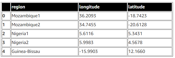\n\nDue to the larger expanse of mangrove forests in Mozambique and Nigeria, two points each are required to capture the respective regions in the preceding table. The full curated list of points is available on [GitHub](https://github.com/aws-samples/mangrove-landcover-classification/blob/e3f501d99f735ae815552dd168d80ab592d86979/data/zones.csv).\n\nTo sample points representing both classes, you have to create a binary mask for each class first. The minority class mask for a Landsat patch is simply the intersection of pixels in the patch and the GMFD dataset. The mask for the majority class for the patch is simply the inverse of the minority class mask. See the following code:\n\n```\\nmangrove_mask = image_patch.updateMask(mangrove_images_landsat.eq(1))\\nnon_mangrove_mask = image_patch.updateMask(mangrove_mask.unmask().Not())\\n```\n\nUse these two masks for the patch and create a set of labeled pixels by randomly sampling pixels from the respective masks:\n\n```\\nmangrove_training_pts = mangrove_mask.sample(**{\\n 'region': mangrove_mask.geometry(),\\n 'scale': 30,\\n 'numPixels': 100000,\\n 'seed': 0,\\n 'geometries': True\\n})\\nnon_mangrove_training_pts = non_mangrove_mask.sample(**{\\n 'region': non_mangrove_mask.geometry(),\\n 'scale': 30,\\n 'numPixels': 50000,\\n 'seed': 0,\\n 'geometries': True\\n})\\n```\n\n```numPixels``` is the number of samples drawn from the entire patch, and the sampled point is retained in the collection only if it falls in the target mask area. Because the mangrove region is typically a small fraction of the Landsat image patch, you need to use a larger value of ```numPixels``` for the mangrove mask compared to that for the non-mangrove mask. You can always look at the size of the two classes as follows to adjust the corresponding ```numPixels``` values:\n\n```\\nmangrove_training_pts.size().getInfo(), non_mangrove_training_pts.size().getInfo()\\n(900, 49500)\\n```\n\nIn this example, the mangrove region is a tiny fraction of the Landsat patch because only 900 points were sampled from 100,000 attempts. Therefore, you should probably increase the value for ```numPixels``` for the minority class to restore balance between the two classes.\n\nIt’s a good idea to visually verify that the sampled points from the two respective sets indeed fall in the intended region in the map:\n\n```\\n# define the point of interest\\nsuriname_lonlat = [-53.94, 5.61]\\nsuriname_point = ee.Geometry.Point(suriname_lonlat)\\ntraining_map = geemap.Map()\\ntraining_map.setCenter(*suriname_lonlat, 13)\\n\\n# define visualization parameters\\nvis_params = {\\n 'min': 0,\\n 'max': 100,\\n 'bands': ['B4']\\n}\\n\\n# define colors for the two set of points\\nmangrove_color = 'eb0000'\\nnon_mangrove_color = '1c5f2c'\\n\\n# create legend for the map\\nlegend_dict = {\\n 'Mangrove Point': mangrove_color,\\n 'Non-mangrove Point': non_mangrove_color\\n}\\n\\n# add layers to the map\\ntraining_map.addLayer(mangrove_mask, vis_params, 'mangrove mask', True)\\ntraining_map.addLayer(mangrove_training_pts, {'color': mangrove_color}, 'Mangrove Sample')\\ntraining_map.addLayer(non_mangrove_mask, {}, 'non mangrove mask', True)\\ntraining_map.addLayer(non_mangrove_training_pts, {'color': non_mangrove_color}, 'non mangrove training', True)\\ntraining_map.add_legend(legend_dict=legend_dict)\\n\\n# display the map\\ntraining_map\\n```\n\nSure enough, as the following image shows, the red points representing mangrove pixels fall in the white regions and the green points representing a lack of mangroves fall in the gray region. The ```maps.ipynb``` [notebook](https://github.com/aws-samples/mangrove-landcover-classification/blob/e3f501d99f735ae815552dd168d80ab592d86979/notebooks/maps.ipynb) walks through the process of generation and visual inspection of sampled points on a map.\n\n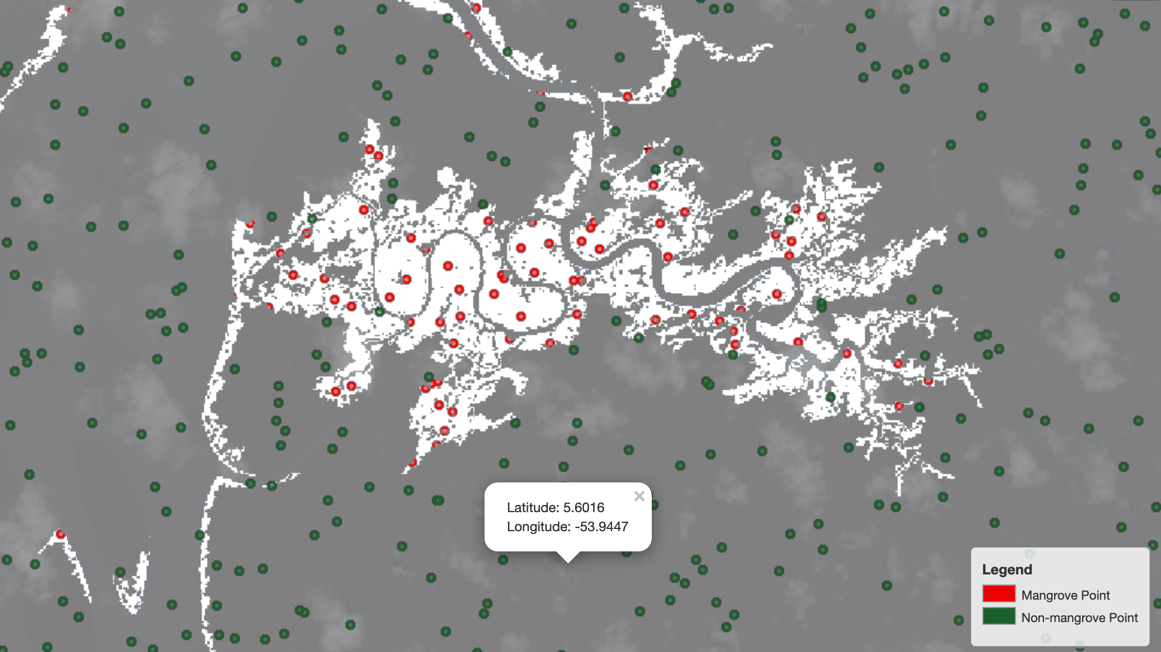\n\nNow you need to convert the sampled points into a DataFrame for ML model training, which can be accomplished by the ```ee_to_geopandas``` module of ```geemap```:\n\n```\\nfrom geemap import ee_to_geopandas\\nmangrove_gdf = ee_to_geopandas(mangrove_training_pts)\\n geometry B1 B2 B3 B4 B5 B6 B7\\n0 POINT (-53.95268 5.73340) 251 326 623 535 1919 970 478\\n1 POINT (-53.38339 5.55982) 4354 4483 4714 4779 5898 4587 3714\\n2 POINT (-53.75469 5.68400) 1229 1249 1519 1455 3279 1961 1454\\n3 POINT (-54.78127 5.95457) 259 312 596 411 3049 1644 740\\n4 POINT (-54.72215 5.97807) 210 279 540 395 2689 1241 510\\n```\n\nThe pixel coordinates at this stage are still represented as a [Shapely](https://autogis-site.readthedocs.io/en/latest/notebooks/L1/geometric-objects.html) geometry point. In the next step, you have to convert those into latitudes and longitudes. Additionally, you need to add labels to the DataFrame, which for the ```mangrove_gdf``` should all be 1, representing the minority class. See the following code:\n\n```\\nmangrove_gdf[\\"lon\\"] = mangrove_gdf[\\"geometry\\"].apply(lambda p: p.x)\\nmangrove_gdf[\\"lat\\"] = mangrove_gdf[\\"geometry\\"].apply(lambda p: p.y)\\nmangrove_gdf[\\"label\\"] = 1 \\nmangrove_gdf = mangrove_gdf.drop(\\"geometry\\", axis=1)\\nprint(mangrove_gdf.head())\\n\\n B1 B2 B3 B4 B5 B6 B7 lon lat label\\n0 251 326 623 535 1919 970 478 -53.952683 5.733402 1\\n1 4354 4483 4714 4779 5898 4587 3714 -53.383394 5.559823 1\\n2 1229 1249 1519 1455 3279 1961 1454 -53.754688 5.683997 1\\n3 259 312 596 411 3049 1644 740 -54.781271 5.954568 1\\n4 210 279 540 395 2689 1241 510 -54.722145 5.978066 1\\n```\n\nSimilarly, create another DataFrame, ```non_mangrove_gdf```, using sampled points from the non-mangrove part of the Landsat image patch and assigning label=0 to all those points. A training dataset for the region is created by appending ```mangrove_gdf``` and ```non_mangrove_gdf```.\n\n### **Exploring the bands**\n\nBefore diving into building a model to classify pixels in an image representing mangroves or not, it’s worth looking into the band values associated with those pixels. There are seven bands in the dataset, and the kernel density plots in the following figure show the distribution of those bands extracted from the 2015 Landsat data for the Indian mangrove region. The distribution of each band is broken down into two groups: pixels representing mangroves, and pixels representing other surface features like water or cultivated land.\n\n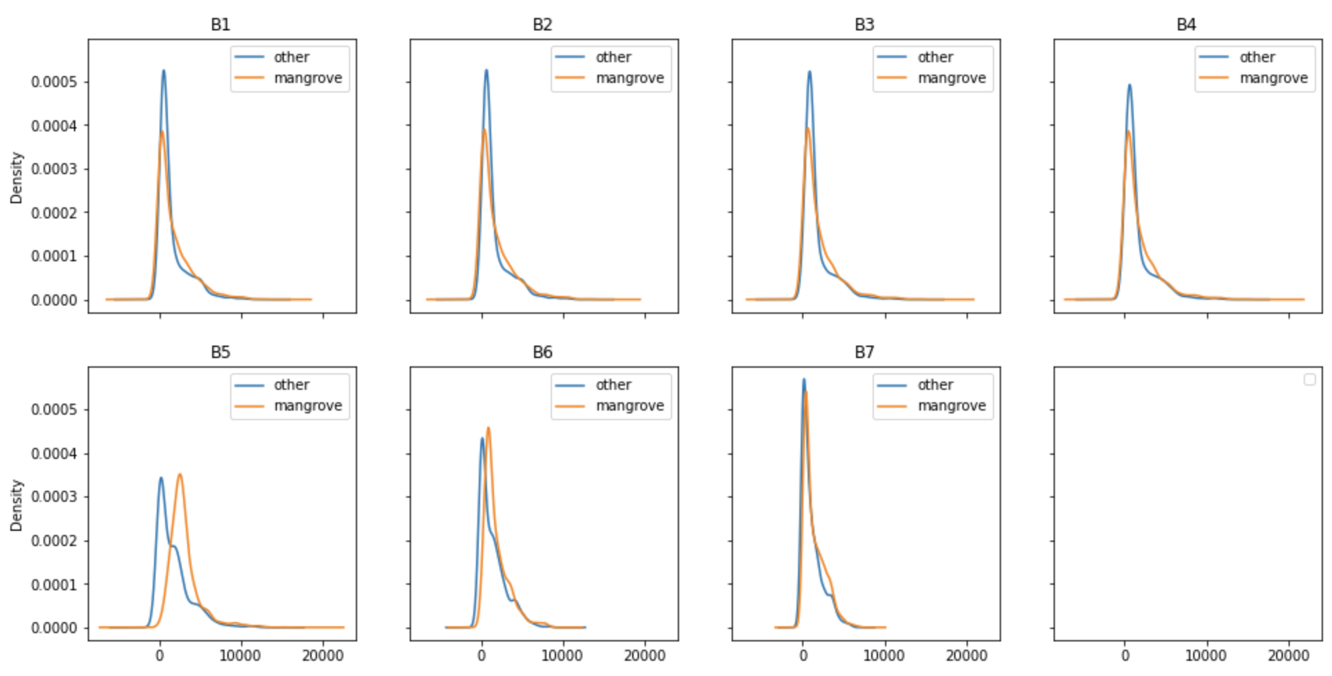\n\nOne important aspect of building a classifier is to understand how these distributions vary over different regions of the Earth. The following figure shows the kernel density plots for bands captured in the same year from the Miami area of the US in 2015. The apparent similarity of the density profiles indicate that it may be possible to build a universal mangrove classifier that can be generalized to predict new areas excluded from the training set.\n\n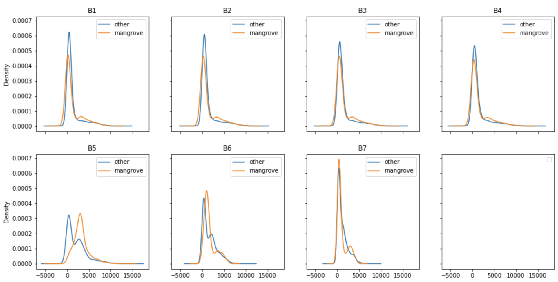\n\nThe plots shown in both figures are generated from band values that represent minimum cloud coverage, as determined by the built-in Earth Engine algorithm. Although this is a very reasonable approach, because different regions on the Earth have varying amounts of cloud coverage on the specific date of data collection, there exist alternative ways to capture the band values. For example, it’s also useful to calculate the median from a [simple composite](https://developers.google.com/earth-engine/guides/landsat#simple-composite) and use it for model training, but those details are beyond the scope of this post.\n\n### **Prepare the training data**\n\nThere are two main strategies to split the labeled dataset into training and test sets. In the first approach, datasets corresponding to the different regions can be combined into a single DataFrame and then split into training and test sets while preserving the fraction of the minority class. The alternative approach is to train a model on a subset of the regions and treat the remaining regions as part of the test set. One of the critical questions we want to address here is how good a model trained in a certain region generalizes over other regions previously unseen. This is important because mangroves from different parts of the world can have some local characteristics, and one way to judge the quality of a model is to investigate how reliable it is in predicting mangrove forests from the satellite image of a new region. Therefore, although splitting the dataset using the first strategy would likely improve the model performance, we follow the second approach.\n\nAs indicated earlier, the mangrove dataset was broken down into geographical regions and four of those, ```Vietnam2```, ```Myanmar3```, ```Cuba2```, and ```India```, were set aside to create the test dataset. The remaining 21 regions made up the training set. The dataset for each region was created by setting ```numPixels=10000``` for mangrove and ```numPixels=1000``` for the non-mangrove regions in the sampling process. The larger value of ```numPixels``` for mangroves ensures a more balanced dataset, because mangroves usually cover a small fraction of the satellite image patches. The resulting training data ended up having a 75/25 split between the majority and minority classes, whereas the split was 69/31 for the test dataset. The regional datasets as well as the training and test datasets were stored in an [Amazon Simple Storage Service](http://aws.amazon.com/s3) ([Amazon S3](https://aws.amazon.com/cn/s3/?trk=cndc-detail)) bucket. The complete code for generating the training and test sets is available in the ```prep_mangrove_dataset.ipynb``` [notebook](https://github.com/aws-samples/mangrove-landcover-classification/blob/e3f501d99f735ae815552dd168d80ab592d86979/notebooks/prep_mangrove_dataset.ipynb).\n\n### **Train a model with smileCart**\n\nOne of the few built-in models GEE provides is a classification and regression tree-based algorithm (smileCart) for quick classification. These built-in models allow you to quickly train a classifier and perform inference, at the cost of detailed model tuning and customization. Even with this downside, using smileCart still provides a beginner-friendly introduction to land cover classification, and therefore can serve as a baseline.\n\nTo train the built-in classifier, you need to provide two pieces of information: the satellite bands to use as features and the column representing the label. Additionally, you have to convert the training and test datasets from Pandas DataFrames to GEE feature collections. Then you instantiate the built-in classifier and train the model. The following is a high-level version of the code; you can find more details in the ```smilecart.ipynb``` [notebook](https://github.com/aws-samples/mangrove-landcover-classification/blob/34d65254015602a98276f2be22fa9995f96357af/notebooks/smilecart.ipynb):\n\n```\\nbands = ['B1', 'B2', 'B3', 'B4', 'B5', 'B6', 'B7']\\nlabel = 'label'\\n\\n# Train a CART classifier with default parameters.\\nclassifier = ee.Classifier.smileCart().train(train_set_pts, label, bands)\\n\\n# Inference on test set\\nresult_featurecollection = test_set_pts.select(bands).classify(classifier)\\n```\n\nBoth ```train_set_pts``` and ```test_set_pts``` are ```FeatureCollections```, a common GEE data structure, containing the train dataset and test dataset, respectively. The model prediction generates the following confusion matrix on the test dataset.\n\n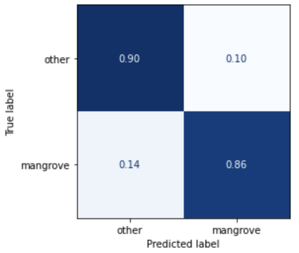\n\nThe model doesn’t predict mangroves very well, but this is a good starting point, and the result will act as a baseline for the custom models you build in part two of this series.\n\n### **Conclusion**\n\nThis concludes the first part of a two-part post, in which we show the ETL process for building a mangrove classifier based on features extracted from satellite images. We showed how to automate the process of gathering satellite images and visualize it in Studio for detailed exploration. In [Part 2](https://aws.amazon.com/blogs/machine-learning/part-2-identify-mangrove-forests-using-satellite-image-features-using-amazon-sagemaker-studio-and-amazon-sagemaker-autopilot/) of the post, we show how to use AutoML to build a custom model in Autopilot that performs better than the built-in smileCart model.\n\n### **About the Authors**\n\n\n\n**Andrei Ivanovic** is an incoming Master’s of Computer Science student at the University of Toronto and a recent graduate of the Engineering Science program at the University of Toronto, majoring in Machine Intelligence with a Robotics/Mechatronics minor. He is interested in computer vision, deep learning, and robotics. He did the work presented in this post during his summer internship at Amazon.\n\n\n\n**David Dong** is a Data Scientist at Amazon Web Services.\n\n\n\n**Arkajyoti Misra** is a Data Scientist at Amazon LastMile Transportation. He is passionate about applying Computer Vision techniques to solve problems that helps the earth. He loves to work with non-profit organizations and is a founding member of ekipi.org.","render":"<p>The increasing ubiquity of satellite data over the last two decades is helping scientists observe and monitor the health of our constantly changing planet. By tracking specific regions of the Earth’s surface, scientists can observe how regions like forests, water bodies, or glaciers change over time. One such region of interest for geologists is mangrove forests. These forests are essential to the overall health of the planet and are one of the many areas across the world that are impacted by human activities. In this post, we show how to get access to satellite imagery data containing mangrove forests and how to visually interact with the data in <ins><a href=\\"https://docs.aws.amazon.com/sagemaker/latest/dg/studio.html\\" target=\\"_blank\\">Amazon SageMaker Studio</a></ins>. In <ins><a href=\\"https://aws.amazon.com/blogs/machine-learning/part-2-identify-mangrove-forests-using-satellite-image-features-using-amazon-sagemaker-studio-and-amazon-sagemaker-autopilot/\\" target=\\"_blank\\">Part 2</a></ins> of this series, we show how to train a machine learning (ML) model using <ins><a href=\\"https://aws.amazon.com/sagemaker/autopilot/\\" target=\\"_blank\\">Amazon SageMaker Autopilot</a></ins> to identify those forests from a satellite image.</p>\n<h3><a id=\\"Overview_of_solution_2\\"></a><strong>Overview of solution</strong></h3>\\n<p>A large number of satellites orbit the Earth, scanning its surface on a regular basis. Typical examples of such satellites are Landsat, Sentinel, CBERS, and MODIS, to name a few. You can access both recent and historical data captured by these satellites at no cost from multiple providers like <a href=\\"https://earthexplorer.usgs.gov/\\" target=\\"_blank\\">USGS EarthExplorer</a>, <a href=\\"https://eos.com/products/landviewer/\\" target=\\"_blank\\">Land Viewer</a>, or <a href=\\"https://scihub.copernicus.eu/\\" target=\\"_blank\\">Copernicus Open Access Hub</a>. Although they provide an excellent service to the scientific community by making their data freely available, it takes a significant amount of effort to gain familiarity with the interfaces of the respective providers. Additionally, such data from satellites is made available in different formats and may not comply with the standard Geographical Information Systems (GIS) data formatting. All of these challenges make it extremely difficult for newcomers to GIS to prepare a suitable dataset for ML model training.</p>\\n<p>Platforms like <a href=\\"https://earthengine.google.com/\\" target=\\"_blank\\">Google Earth Engine</a> (GEE) and <a href=\\"https://aws.amazon.com/earth/\\" target=\\"_blank\\">Earth on AWS</a> make a wide variety of satellite imagery data available in a single portal that eases searching for the right dataset and standardizes the ETL (extract, transform, and load) component of the ML workflow in a convenient, beginner-friendly manner. GEE additionally provides a coding platform where you can programmatically explore the dataset and build a model in JavaScript. The Python API for GEE lacks the maturity of its JavaScript counterpart; however, that gap is sufficiently bridged by the open-sourced project geemap.</p>\\n<p>In this series of posts, we present a complete end-to-end example of building an ML model in the GIS space to detect mangrove forests from satellite images. Our goal is to provide a template solution that ML engineers and data scientists can use to explore and interact with the satellite imagery, make the data available in the right format for building a classifier, and have the option to validate model predictions visually. Specifically, we walk through the following:</p>\n<ul>\\n<li>How to download satellite imagery data to a Studio environment</li>\n<li>How to interact with satellite data and perform exploratory data analysis in a Studio notebook</li>\n<li>How to automate training an ML model in Autopilot</li>\n</ul>\\n<h3><a id=\\"Build_the_environment_14\\"></a><strong>Build the environment</strong></h3>\\n<p>The solution presented in this post is built in a Studio environment. To configure the environment, complete the following steps:</p>\n<ol>\\n<li>Add a new SageMaker domain user and launch the Studio app. (For instructions, refer to <a href=\\"https://docs.aws.amazon.com/sagemaker/latest/dg/notebooks-get-started.html\\" target=\\"_blank\\">Get Started</a>.)</li>\\n<li>Open a new Studio notebook by choosing the plus sign under <strong>Notebook and compute resources</strong> (make sure to choose the Data Science SageMaker image).</li>\\n</ol>\n<p><img src=\\"https://dev-media.amazoncloud.cn/bbec6b11029a4a3cb80f5605537b584f_image.png\\" alt=\\"image.png\\" /></p>\n<ol start=\\"3\\">\\n<li>Clone the <a href=\\"https://github.com/aws-samples/mangrove-landcover-classification\\" target=\\"_blank\\">mangrove-landcover-classification</a> Git repository, which contains all the code used for this post. (For instructions, refer to <a href=\\"https://docs.aws.amazon.com/sagemaker/latest/dg/studio-tasks-git.html\\" target=\\"_blank\\">Clone a Git Repository in SageMaker Studio</a>).</li>\\n<li>Open the<br />\\nnotebook <code>notebooks/explore_mangrove_data.ipynb</code>.</li>\\n<li>Run the first notebook cell to pip install all the required dependencies listed in the requirements.txt file in the root folder.</li>\n<li>Open a new Launcher tab and open a system terminal found in the Utilities and files section.</li>\n</ol>\\n<p><img src=\\"https://dev-media.amazoncloud.cn/c58f773c2d664e5cafe0ddad5d7064f8_image.png\\" alt=\\"image.png\\" /></p>\n<ol start=\\"7\\">\\n<li>Install the Earth Engine API:</li>\n</ol>\\n<pre><code class=\\"lang-\\">pip install earthengine-api\\n</code></pre>\\n<ol start=\\"8\\">\\n<li>Authenticate Earth Engine:</li>\n</ol>\\n<pre><code class=\\"lang-\\">earthengine authenticate\\n</code></pre>\\n<p><img src=\\"https://dev-media.amazoncloud.cn/51fa465423c34673baf9bbe3a57ba9c8_image.png\\" alt=\\"image.png\\" /></p>\n<ol start=\\"9\\">\\n<li>Follow the Earth Engine link in the output and <a href=\\"https://earthengine.google.com/signup/\\" target=\\"_blank\\">sign up</a> as a developer so that you can access GIS data from a notebook.</li>\\n</ol>\n<h3><a id=\\"Mangrove_dataset_47\\"></a><strong>Mangrove dataset</strong></h3>\\n<p>The <a href=\\"https://developers.google.com/earth-engine/datasets/catalog/LANDSAT_MANGROVE_FORESTS\\" target=\\"_blank\\">Global Mangrove Forest Distribution</a> (GMFD) is one of the most cited datasets used by researchers in the area. The dataset, which contains labeled mangrove regions at a 30-meter resolution from around the world, is curated from more than 1,000 <a href=\\"https://landsat.gsfc.nasa.gov/\\" target=\\"_blank\\">Landsat</a> images obtained from the <a href=\\"https://www.usgs.gov/centers/eros\\" target=\\"_blank\\">USGS EROS</a> Center. One of the disadvantages of using the dataset is that it was compiled in 2000. In the absence of a newer dataset that is as comprehensive as the GMFD, we decided to use it because it serves the purpose of demonstrating an ML workload in the GIS space.</p>\\n<p>Given the visual nature of GIS data, it’s critical for ML practitioners to be able to interact with satellite images in an interactive manner with full map functionalities. Although GEE provides this functionality through a <a href=\\"https://code.earthengine.google.com/\\" target=\\"_blank\\">browser interface</a>, it’s only available in JavaScript. Fortunately, the open-sourced project geemap aids data scientists by providing those functionalities in Python.</p>\\n<p>Go back to the <code>explore_mangrove_data.ipynb</code> notebook you opened earlier and follow the remaining cells to understand how to use simple interactive maps in the notebook.</p>\\n<ol>\\n<li>Start by importing Earth Engine and initializing it:</li>\n</ol>\\n<pre><code class=\\"lang-\\">import ee\\nimport geemap.eefolium as geemap\\nee.Initialize()\\n</code></pre>\\n<ol start=\\"2\\">\\n<li>Now import the satellite image collection from the database:</li>\n</ol>\\n<pre><code class=\\"lang-\\">mangrove_images_landsat = ee.ImageCollection('LANDSAT/MANGROVE_FORESTS')\\n</code></pre>\\n<ol start=\\"3\\">\\n<li>Extract the collection, which contains just one set:</li>\n</ol>\\n<pre><code class=\\"lang-\\">mangrove_images_landsat = mangrove_images_landsat.first()\\n</code></pre>\\n<ol start=\\"4\\">\\n<li>To visualize the data on a map, you first need to instantiate a map through geemap:</li>\n</ol>\\n<pre><code class=\\"lang-\\">mangrove_map = geemap.Map()\\n</code></pre>\\n<ol start=\\"5\\">\\n<li>Next, define some parameters that make it easy to visualize the data on a world map:</li>\n</ol>\\n<pre><code class=\\"lang-\\">mangrovesVis = {\\n min: 0,\\n max: 1.0,\\n 'palette': ['d40115'],\\n }\\n</code></pre>\\n<ol start=\\"6\\">\\n<li>Now add the data as a layer on the map instantiated earlier with the visualization parameters:</li>\n</ol>\\n<pre><code class=\\"lang-\\">mangrove_map.addLayer(mangrove_images_landsat, mangrovesVis, 'Mangroves')\\n</code></pre>\\n<p>You can add as many layers as you want to the map and then interactively turn them on or off for a cleaner view when necessary. Because mangrove forests aren’t everywhere on the earth, it makes sense to center the map to a coastal region with known mangrove forests and then render the map on the notebook as follows:</p>\n<pre><code class=\\"lang-\\">mangrove_map.setCenter(-81, 25, 9)\\nmangrove_map\\n</code></pre>\\n<p>The latitude and longitude chosen here, 25 degrees north and 81 degrees west, respectively, correspond to the gulf coast of Florida, US. The map is rendered at a zoom level of 9, where a higher number provides a more closeup view.</p>\n<p><img src=\\"https://dev-media.amazoncloud.cn/385782f16471434fa516d384a12c26cb_image.png\\" alt=\\"image.png\\" /></p>\n<p>You can obtain some useful information about the dataset by accessing the associated metadata as follows:</p>\n<pre><code class=\\"lang-\\">geemap.image_props(mangrove_images_landsat).getInfo()\\n</code></pre>\\n<p>You get the following output:</p>\n<pre><code class=\\"lang-\\">{'IMAGE_DATE': '2000-01-01',\\n 'NOMINAL_SCALE': 30.359861978395436,\\n 'system:asset_size': '41.133541 MB',\\n 'system:band_names': ['1'],\\n 'system:id': 'LANDSAT/MANGROVE_FORESTS/2000',\\n 'system:index': '2000',\\n 'system:time_end': '2001-01-01 00:00:00',\\n 'system:time_start': '2000-01-01 00:00:00',\\n 'system:version': 1506796895089836\\n}\\n</code></pre>\\n<p>Most of the fields in the metadata are self-explanatory, except for the band names. The next section discusses this field in more detail.</p>\n<h3><a id=\\"Landsat_dataset_131\\"></a><strong>Landsat dataset</strong></h3>\\n<p>The following image is a satellite image of an area at the border of French Guiana and Suriname, where mangrove forests are common. The left image shows a raw satellite image of the region; the image on the right depicts the GMFD data superimposed on it. Pixels representing mangroves are shown in red. It’s quite evident from the side-by-side comparison that there is no straightforward visual cue in either structure or color in the underlying satellite image that distinguishes mangroves from the surrounding region. In the absence of any such distinguishing pattern in the images, it poses a considerable challenge even for state-of-the-art deep learning-based classifiers to identify mangroves accurately. Fortunately, satellite images are captured at a range of wavelengths on the electromagnetic spectrum, part of which falls outside the visible range. Additionally, they also contain important measurements like surface reflectance. Therefore, researchers in the field have traditionally relied upon these measurements to build ML classifiers.</p>\n<p><img src=\\"https://dev-media.amazoncloud.cn/cb81ea0cfc0f410b90fff50b55b0cb4b_image.png\\" alt=\\"image.png\\" /></p>\n<p>Unfortunately, apart from marking whether or not an individual pixel represents mangroves, the GMFD dataset doesn’t provide any additional information. However, other datasets can provide a host of features for every pixel that can be utilized to train a classifier. In this post, you use the <a href=\\"https://www.usgs.gov/core-science-systems/nli/landsat/landsat-surface-reflectance?qt-science_support_page_related_con=0#qt-science_support_page_related_con\\" target=\\"_blank\\">USGS Landsat 8 dataset</a> for that purpose. The <a href=\\"https://www.usgs.gov/core-science-systems/nli/landsat/landsat-8?qt-science_support_page_related_con=0\\" target=\\"_blank\\">Landsat 8</a> satellite was launched in 2013 and orbits the Earth every 99 minutes at an altitude of 705 km, capturing images covering a 185 km x 180 km patch on the Earth’s surface. It captures nine spectral bands, or portions of the electromagnetic spectrum sensed by a satellite, ranging from ultra blue to shortwave infrared. Therefore, the images available in the Landsat dataset are a collection of image patches containing multiple bands, with each patch time stamped by the date of collection.</p>\\n<p>To get a sample image from the Landsat dataset, you need to define a point of interest:</p>\n<pre><code class=\\"lang-\\">point = ee.Geometry.Point([&lt;longitude&gt;, &lt;latitude&gt;])\\n</code></pre>\\n<p>Then you filter the image collection by the point of interest, a date range, and optionally by the bands of interest. Because the images collected by the satellites are often obscured by cloud cover, it’s absolutely necessary to extract images with the minimum amount of cloud cover. Fortunately, the Landsat dataset already comes with a cloud detector. This streamlines the process of accessing all available images over several months, sorting them by amount of cloud cover, and picking the one with minimum cloud cover. For example, you can perform the entire process of extracting a Landsat image patch from the northern coast of the continent of South America in a few lines of code:</p>\n<pre><code class=\\"lang-\\">point = ee.Geometry.Point([-53.94, 5.61])\\nimage_patch = ee.ImageCollection('LANDSAT/LC08/C01/T1_SR') \\\\\\n .filterBounds(point) \\\\\\n .filterDate('2016-01-01', '2016-12-31') \\\\\\n .select('B[1-7]') \\\\\\n .sort('CLOUD_COVER') \\\\\\n .first()\\n</code></pre>\\n<p>When specifying a region using a point of interest, that region doesn’t necessarily have to be centered on that point. The extracted image patch simply contains the point somewhere within it.</p>\n<p>Finally, you can plot the image patch over a map by specifying proper plotting parameters based on a few of the chosen bands:</p>\n<pre><code class=\\"lang-\\">vis_params = {\\n \\t\\t\\t'min': 0,\\n'max': 3000,\\n'bands': ['B5', 'B4', 'B3']\\n }\\nlandsat = geemap.Map()\\nlandsat.centerObject(point, 8)\\nlandsat.addLayer(image_patch, vis_params, &quot;Landsat-8&quot;)\\nlandsat\\n</code></pre>\\n<p>The following is a sample image patch collected by Landsat 8 showing in false color the Suriname-French Guiana border region. The mangrove regions are too tiny to be visible at the scale of the image.</p>\n<p><img src=\\"https://dev-media.amazoncloud.cn/13dc0dbc4585489b8458b125f9999784_image.png\\" alt=\\"image.png\\" /></p>\n<p>As usual, there is a host of useful metadata available for the extracted image:</p>\n<pre><code class=\\"lang-\\">geemap.image_props(image_patch).getInfo()\\n\\n{'CLOUD_COVER': 5.76,\\n 'CLOUD_COVER_LAND': 8.93,\\n 'EARTH_SUN_DISTANCE': 0.986652,\\n 'ESPA_VERSION': '2_23_0_1a',\\n 'GEOMETRIC_RMSE_MODEL': 9.029,\\n 'GEOMETRIC_RMSE_MODEL_X': 6.879,\\n 'GEOMETRIC_RMSE_MODEL_Y': 5.849,\\n 'IMAGE_DATE': '2016-11-27',\\n 'IMAGE_QUALITY_OLI': 9,\\n 'IMAGE_QUALITY_TIRS': 9,\\n 'LANDSAT_ID': 'LC08_L1TP_228056_20161127_20170317_01_T1',\\n 'LEVEL1_PRODUCTION_DATE': 1489783959000,\\n 'NOMINAL_SCALE': 30,\\n 'PIXEL_QA_VERSION': 'generate_pixel_qa_1.6.0',\\n 'SATELLITE': 'LANDSAT_8',\\n 'SENSING_TIME': '2016-11-27T13:52:20.6150480Z',\\n 'SOLAR_AZIMUTH_ANGLE': 140.915802,\\n 'SOLAR_ZENITH_ANGLE': 35.186565,\\n 'SR_APP_VERSION': 'LaSRC_1.3.0',\\n 'WRS_PATH': 228,\\n 'WRS_ROW': 56,\\n 'system:asset_size': '487.557501 MB',\\n 'system:band_names': ['B1', 'B2', 'B3', 'B4', 'B5', 'B6', 'B7'],\\n 'system:id': 'LANDSAT/LC08/C01/T1_SR/LC08_228056_20161127',\\n 'system:index': 'LC08_228056_20161127',\\n 'system:time_end': '2016-11-27 13:52:20',\\n 'system:time_start': '2016-11-27 13:52:20',\\n 'system:version': 1522722936827122}\\n</code></pre>\\n<p>The preceding image isn’t free from clouds, which is confirmed by the metadata suggesting a 5.76% cloud cover. Compared to a single binary band available from the GMFD image, the Landsat image contains the bands B1–B7.</p>\n<h3><a id=\\"ETL_process_214\\"></a><strong>ETL process</strong></h3>\\n<p>To summarize, you need to work with two distinct datasets to train a mangrove classifier. The GMFD dataset provides only the coordinates of pixels belonging to the minority class (mangrove). The Landsat dataset, on the other hand, provides band information for every pixel in a collection of patches, each patch covering roughly a 180 km2 area on the Earth’s surface. You now need to combine these two datasets to create the training dataset containing pixels belonging to both the minority and majority classes.</p>\n<p>It’s wasteful to have a training dataset covering the entire surface of the Earth, because the mangrove regions cover a tiny fraction of the surface area. Because these regions are generally isolated from one another, an effective strategy is to create a set of points, each representing a specific mangrove forest on the earth’s surface, and collect the Landsat patches around those points. Subsequently, pixels can be sampled from each Landsat patch and a class—either mangrove or non-mangrove—can be assigned to it depending on whether the pixel appears in the GMFD dataset. The full labeled dataset can then be constructed by aggregating points sampled from this collection of patches.</p>\n<p>The following table shows a sample of the regions and the corresponding coordinates to filter the Landsat patches.</p>\n<p><img src=\\"https://dev-media.amazoncloud.cn/b4c718be487546fb8f0df163bd07fd28_image.png\\" alt=\\"image.png\\" /></p>\n<p>Due to the larger expanse of mangrove forests in Mozambique and Nigeria, two points each are required to capture the respective regions in the preceding table. The full curated list of points is available on <a href=\\"https://github.com/aws-samples/mangrove-landcover-classification/blob/e3f501d99f735ae815552dd168d80ab592d86979/data/zones.csv\\" target=\\"_blank\\">GitHub</a>.</p>\\n<p>To sample points representing both classes, you have to create a binary mask for each class first. The minority class mask for a Landsat patch is simply the intersection of pixels in the patch and the GMFD dataset. The mask for the majority class for the patch is simply the inverse of the minority class mask. See the following code:</p>\n<pre><code class=\\"lang-\\">mangrove_mask = image_patch.updateMask(mangrove_images_landsat.eq(1))\\nnon_mangrove_mask = image_patch.updateMask(mangrove_mask.unmask().Not())\\n</code></pre>\\n<p>Use these two masks for the patch and create a set of labeled pixels by randomly sampling pixels from the respective masks:</p>\n<pre><code class=\\"lang-\\">mangrove_training_pts = mangrove_mask.sample(**{\\n 'region': mangrove_mask.geometry(),\\n 'scale': 30,\\n 'numPixels': 100000,\\n 'seed': 0,\\n 'geometries': True\\n})\\nnon_mangrove_training_pts = non_mangrove_mask.sample(**{\\n 'region': non_mangrove_mask.geometry(),\\n 'scale': 30,\\n 'numPixels': 50000,\\n 'seed': 0,\\n 'geometries': True\\n})\\n</code></pre>\\n<p><code>numPixels</code> is the number of samples drawn from the entire patch, and the sampled point is retained in the collection only if it falls in the target mask area. Because the mangrove region is typically a small fraction of the Landsat image patch, you need to use a larger value of <code>numPixels</code> for the mangrove mask compared to that for the non-mangrove mask. You can always look at the size of the two classes as follows to adjust the corresponding <code>numPixels</code> values:</p>\\n<pre><code class=\\"lang-\\">mangrove_training_pts.size().getInfo(), non_mangrove_training_pts.size().getInfo()\\n(900, 49500)\\n</code></pre>\\n<p>In this example, the mangrove region is a tiny fraction of the Landsat patch because only 900 points were sampled from 100,000 attempts. Therefore, you should probably increase the value for <code>numPixels</code> for the minority class to restore balance between the two classes.</p>\\n<p>It’s a good idea to visually verify that the sampled points from the two respective sets indeed fall in the intended region in the map:</p>\n<pre><code class=\\"lang-\\"># define the point of interest\\nsuriname_lonlat = [-53.94, 5.61]\\nsuriname_point = ee.Geometry.Point(suriname_lonlat)\\ntraining_map = geemap.Map()\\ntraining_map.setCenter(*suriname_lonlat, 13)\\n\\n# define visualization parameters\\nvis_params = {\\n 'min': 0,\\n 'max': 100,\\n 'bands': ['B4']\\n}\\n\\n# define colors for the two set of points\\nmangrove_color = 'eb0000'\\nnon_mangrove_color = '1c5f2c'\\n\\n# create legend for the map\\nlegend_dict = {\\n 'Mangrove Point': mangrove_color,\\n 'Non-mangrove Point': non_mangrove_color\\n}\\n\\n# add layers to the map\\ntraining_map.addLayer(mangrove_mask, vis_params, 'mangrove mask', True)\\ntraining_map.addLayer(mangrove_training_pts, {'color': mangrove_color}, 'Mangrove Sample')\\ntraining_map.addLayer(non_mangrove_mask, {}, 'non mangrove mask', True)\\ntraining_map.addLayer(non_mangrove_training_pts, {'color': non_mangrove_color}, 'non mangrove training', True)\\ntraining_map.add_legend(legend_dict=legend_dict)\\n\\n# display the map\\ntraining_map\\n</code></pre>\\n<p>Sure enough, as the following image shows, the red points representing mangrove pixels fall in the white regions and the green points representing a lack of mangroves fall in the gray region. The <code>maps.ipynb</code> <a href=\\"https://github.com/aws-samples/mangrove-landcover-classification/blob/e3f501d99f735ae815552dd168d80ab592d86979/notebooks/maps.ipynb\\" target=\\"_blank\\">notebook</a> walks through the process of generation and visual inspection of sampled points on a map.</p>\\n<p><img src=\\"https://dev-media.amazoncloud.cn/c046af02678d4acc87f7f9ca84849437_image.png\\" alt=\\"image.png\\" /></p>\n<p>Now you need to convert the sampled points into a DataFrame for ML model training, which can be accomplished by the <code>ee_to_geopandas</code> module of <code>geemap</code>:</p>\\n<pre><code class=\\"lang-\\">from geemap import ee_to_geopandas\\nmangrove_gdf = ee_to_geopandas(mangrove_training_pts)\\n geometry B1 B2 B3 B4 B5 B6 B7\\n0 POINT (-53.95268 5.73340) 251 326 623 535 1919 970 478\\n1 POINT (-53.38339 5.55982) 4354 4483 4714 4779 5898 4587 3714\\n2 POINT (-53.75469 5.68400) 1229 1249 1519 1455 3279 1961 1454\\n3 POINT (-54.78127 5.95457) 259 312 596 411 3049 1644 740\\n4 POINT (-54.72215 5.97807) 210 279 540 395 2689 1241 510\\n</code></pre>\\n<p>The pixel coordinates at this stage are still represented as a <a href=\\"https://autogis-site.readthedocs.io/en/latest/notebooks/L1/geometric-objects.html\\" target=\\"_blank\\">Shapely</a> geometry point. In the next step, you have to convert those into latitudes and longitudes. Additionally, you need to add labels to the DataFrame, which for the <code>mangrove_gdf</code> should all be 1, representing the minority class. See the following code:</p>\\n<pre><code class=\\"lang-\\">mangrove_gdf[&quot;lon&quot;] = mangrove_gdf[&quot;geometry&quot;].apply(lambda p: p.x)\\nmangrove_gdf[&quot;lat&quot;] = mangrove_gdf[&quot;geometry&quot;].apply(lambda p: p.y)\\nmangrove_gdf[&quot;label&quot;] = 1 \\nmangrove_gdf = mangrove_gdf.drop(&quot;geometry&quot;, axis=1)\\nprint(mangrove_gdf.head())\\n\\n B1 B2 B3 B4 B5 B6 B7 lon lat label\\n0 251 326 623 535 1919 970 478 -53.952683 5.733402 1\\n1 4354 4483 4714 4779 5898 4587 3714 -53.383394 5.559823 1\\n2 1229 1249 1519 1455 3279 1961 1454 -53.754688 5.683997 1\\n3 259 312 596 411 3049 1644 740 -54.781271 5.954568 1\\n4 210 279 540 395 2689 1241 510 -54.722145 5.978066 1\\n</code></pre>\\n<p>Similarly, create another DataFrame, <code>non_mangrove_gdf</code>, using sampled points from the non-mangrove part of the Landsat image patch and assigning label=0 to all those points. A training dataset for the region is created by appending <code>mangrove_gdf</code> and <code>non_mangrove_gdf</code>.</p>\\n<h3><a id=\\"Exploring_the_bands_334\\"></a><strong>Exploring the bands</strong></h3>\\n<p>Before diving into building a model to classify pixels in an image representing mangroves or not, it’s worth looking into the band values associated with those pixels. There are seven bands in the dataset, and the kernel density plots in the following figure show the distribution of those bands extracted from the 2015 Landsat data for the Indian mangrove region. The distribution of each band is broken down into two groups: pixels representing mangroves, and pixels representing other surface features like water or cultivated land.</p>\n<p><img src=\\"https://dev-media.amazoncloud.cn/8b3bc7c8e79d440a9b362ec6ead8f402_image.png\\" alt=\\"image.png\\" /></p>\n<p>One important aspect of building a classifier is to understand how these distributions vary over different regions of the Earth. The following figure shows the kernel density plots for bands captured in the same year from the Miami area of the US in 2015. The apparent similarity of the density profiles indicate that it may be possible to build a universal mangrove classifier that can be generalized to predict new areas excluded from the training set.</p>\n<p><img src=\\"https://dev-media.amazoncloud.cn/8de99704f7494422a04c06d76620a987_image.png\\" alt=\\"image.png\\" /></p>\n<p>The plots shown in both figures are generated from band values that represent minimum cloud coverage, as determined by the built-in Earth Engine algorithm. Although this is a very reasonable approach, because different regions on the Earth have varying amounts of cloud coverage on the specific date of data collection, there exist alternative ways to capture the band values. For example, it’s also useful to calculate the median from a <a href=\\"https://developers.google.com/earth-engine/guides/landsat#simple-composite\\" target=\\"_blank\\">simple composite</a> and use it for model training, but those details are beyond the scope of this post.</p>\\n<h3><a id=\\"Prepare_the_training_data_346\\"></a><strong>Prepare the training data</strong></h3>\\n<p>There are two main strategies to split the labeled dataset into training and test sets. In the first approach, datasets corresponding to the different regions can be combined into a single DataFrame and then split into training and test sets while preserving the fraction of the minority class. The alternative approach is to train a model on a subset of the regions and treat the remaining regions as part of the test set. One of the critical questions we want to address here is how good a model trained in a certain region generalizes over other regions previously unseen. This is important because mangroves from different parts of the world can have some local characteristics, and one way to judge the quality of a model is to investigate how reliable it is in predicting mangrove forests from the satellite image of a new region. Therefore, although splitting the dataset using the first strategy would likely improve the model performance, we follow the second approach.</p>\n<p>As indicated earlier, the mangrove dataset was broken down into geographical regions and four of those, <code>Vietnam2</code>, <code>Myanmar3</code>, <code>Cuba2</code>, and <code>India</code>, were set aside to create the test dataset. The remaining 21 regions made up the training set. The dataset for each region was created by setting <code>numPixels=10000</code> for mangrove and <code>numPixels=1000</code> for the non-mangrove regions in the sampling process. The larger value of <code>numPixels</code> for mangroves ensures a more balanced dataset, because mangroves usually cover a small fraction of the satellite image patches. The resulting training data ended up having a 75/25 split between the majority and minority classes, whereas the split was 69/31 for the test dataset. The regional datasets as well as the training and test datasets were stored in an <a href=\\"http://aws.amazon.com/s3\\" target=\\"_blank\\">Amazon Simple Storage Service</a> ([Amazon S3](https://aws.amazon.com/cn/s3/?trk=cndc-detail)) bucket. The complete code for generating the training and test sets is available in the <code>prep_mangrove_dataset.ipynb</code> <a href=\\"https://github.com/aws-samples/mangrove-landcover-classification/blob/e3f501d99f735ae815552dd168d80ab592d86979/notebooks/prep_mangrove_dataset.ipynb\\" target=\\"_blank\\">notebook</a>.</p>\\n<h3><a id=\\"Train_a_model_with_smileCart_352\\"></a><strong>Train a model with smileCart</strong></h3>\\n<p>One of the few built-in models GEE provides is a classification and regression tree-based algorithm (smileCart) for quick classification. These built-in models allow you to quickly train a classifier and perform inference, at the cost of detailed model tuning and customization. Even with this downside, using smileCart still provides a beginner-friendly introduction to land cover classification, and therefore can serve as a baseline.</p>\n<p>To train the built-in classifier, you need to provide two pieces of information: the satellite bands to use as features and the column representing the label. Additionally, you have to convert the training and test datasets from Pandas DataFrames to GEE feature collections. Then you instantiate the built-in classifier and train the model. The following is a high-level version of the code; you can find more details in the <code>smilecart.ipynb</code> <a href=\\"https://github.com/aws-samples/mangrove-landcover-classification/blob/34d65254015602a98276f2be22fa9995f96357af/notebooks/smilecart.ipynb\\" target=\\"_blank\\">notebook</a>:</p>\\n<pre><code class=\\"lang-\\">bands = ['B1', 'B2', 'B3', 'B4', 'B5', 'B6', 'B7']\\nlabel = 'label'\\n\\n# Train a CART classifier with default parameters.\\nclassifier = ee.Classifier.smileCart().train(train_set_pts, label, bands)\\n\\n# Inference on test set\\nresult_featurecollection = test_set_pts.select(bands).classify(classifier)\\n</code></pre>\\n<p>Both <code>train_set_pts</code> and <code>test_set_pts</code> are <code>FeatureCollections</code>, a common GEE data structure, containing the train dataset and test dataset, respectively. The model prediction generates the following confusion matrix on the test dataset.</p>\\n<p><img src=\\"https://dev-media.amazoncloud.cn/6e41ad0894554b42a98f512d0b0bea92_image.png\\" alt=\\"image.png\\" /></p>\n<p>The model doesn’t predict mangroves very well, but this is a good starting point, and the result will act as a baseline for the custom models you build in part two of this series.</p>\n<h3><a id=\\"Conclusion_375\\"></a><strong>Conclusion</strong></h3>\\n<p>This concludes the first part of a two-part post, in which we show the ETL process for building a mangrove classifier based on features extracted from satellite images. We showed how to automate the process of gathering satellite images and visualize it in Studio for detailed exploration. In <a href=\\"https://aws.amazon.com/blogs/machine-learning/part-2-identify-mangrove-forests-using-satellite-image-features-using-amazon-sagemaker-studio-and-amazon-sagemaker-autopilot/\\" target=\\"_blank\\">Part 2</a> of the post, we show how to use AutoML to build a custom model in Autopilot that performs better than the built-in smileCart model.</p>\\n<h3><a id=\\"About_the_Authors_379\\"></a><strong>About the Authors</strong></h3>\\n<p><img src=\\"https://dev-media.amazoncloud.cn/d4a10c5416b54d4c842ad60d375826fe_image.png\\" alt=\\"image.png\\" /></p>\n<p><strong>Andrei Ivanovic</strong> is an incoming Master’s of Computer Science student at the University of Toronto and a recent graduate of the Engineering Science program at the University of Toronto, majoring in Machine Intelligence with a Robotics/Mechatronics minor. He is interested in computer vision, deep learning, and robotics. He did the work presented in this post during his summer internship at Amazon.</p>\\n<p><img src=\\"https://dev-media.amazoncloud.cn/651359ff15124fae98fa3e671c58333f_image.png\\" alt=\\"image.png\\" /></p>\n<p><strong>David Dong</strong> is a Data Scientist at Amazon Web Services.</p>\\n<p><img src=\\"https://dev-media.amazoncloud.cn/866a42f4ba1f4f4b98edd8b98f25afe0_image.png\\" alt=\\"image.png\\" /></p>\n<p><strong>Arkajyoti Misra</strong> is a Data Scientist at Amazon LastMile Transportation. He is passionate about applying Computer Vision techniques to solve problems that helps the earth. He loves to work with non-profit organizations and is a founding member of ekipi.org.</p>\n"}