Feature engineering at scale for healthcare and life sciences with Amazon SageMaker Data Wrangler

{"value":"Machine learning (ML) is disrupting a lot of industries at an unprecedented pace. The healthcare and life sciences (HCLS) industry has been going through a rapid evolution in recent years embracing ML across a multitude of use cases for delivering quality care and improving patient outcomes.\n\nIn a typical ML lifecycle, data engineers and scientists spend the majority of their time on the data preparation and feature engineering steps before even getting started with the process of model building and training. Having a tool that can lower the barrier to entry for data preparation, thereby improving productivity, is a highly desirable ask for these personas. [Amazon SageMaker Data Wrangler](https://docs.aws.amazon.com/sagemaker/latest/dg/data-wrangler.html) is purpose built by AWS to reduce the learning curve and enable data practitioners to accomplish data preparation, cleaning, and feature engineering tasks in less effort and time. It offers a GUI interface with many built-in functions and integrations with other AWS services such as [Amazon Simple Storage Service](https://aws.amazon.com/cn/s3/) ([Amazon S3](https://aws.amazon.com/cn/s3/?trk=cndc-detail)) and [Amazon SageMaker Feature Store](https://aws.amazon.com/cn/sagemaker/feature-store/), as well as partner data sources including Snowflake and Databricks.\n\nIn this post, we demonstrate how to use Data Wrangler to prepare healthcare data for training a model to predict heart failure, given a patient’s demographics, prior medical conditions, and lab test result history.\n\n#### **Solution overview**\n\nThe solution consists of the following steps:\n\n1. Acquire a healthcare dataset as input to Data Wrangler.\n2. Use Data Wrangler’s built-in transformation functions to transform the dataset. This includes drop columns, featurize data/time, join datasets, impute missing values, encode categorical variables, scale numeric values, balance the dataset, and more.\n3. Use Data Wrangler’s custom transform function (Pandas or PySpark code) to supplement additional transformations required beyond the built-in transformations and demonstrate the extensibility of Data Wrangler. This includes filter rows, group data, form new dataframes based on conditions, and more.\n4. Use Data Wrangler’s built-in visualization functions to perform visual analysis. This includes target leakage, feature correlation, quick model, and more.\n5. Use Data Wrangler’s built-in export options to export the transformed dataset to [Amazon S3](https://aws.amazon.com/cn/s3/?trk=cndc-detail).\n6. Launch a Jupyter notebook to use the transformed dataset in [Amazon S3](https://aws.amazon.com/cn/s3/?trk=cndc-detail) as input to train a model.\n\n#### **Generate a dataset**\n\nNow that we have settled on the ML problem statement, we first set our sights on acquiring the data we need. Research studies such as [Heart Failure Prediction](https://www.kaggle.com/datasets/andrewmvd/heart-failure-clinical-data) may provide data that’s already in good shape. However, we often encounter scenarios where the data is quite messy and requires joining, cleansing, and several other transformations that are very specific to the healthcare domain before it can be used for ML training. We want to find or generate data that is messy enough and walk you through the steps of preparing it using Data Wrangler. With that in mind, we picked Synthea as a tool to generate synthetic data that fits our goal. [Synthea](https://github.com/synthetichealth/synthea) is an open-source synthetic patient generator that models the medical history of synthetic patients. To generate your dataset, complete the following steps:\n\n1. Follow the instructions as per the [quick start](https://docs.aws.amazon.com/sagemaker/latest/dg/onboard-quick-start.html) documentation to create an [Amazon SageMaker Studio](https://aws.amazon.com/cn/sagemaker/studio/) domain and launch Studio.\nThis is a prerequisite step. It is optional if Studio is already set up in your account.\n2. After Studio is launched, on the **Launcher** tab, choose **System terminal**.\nThis launches a terminal session that gives you a command line interface to work with.\n\n\n3. To install Synthea and generate the dataset in CSV format, run the following commands in the launched terminal session:\n\n```\\n\$ sudo yum install -y java-1.8.0-openjdk-devel\\n\$ export JAVA_HOME=/usr/lib/jvm/jre-1.8.0-openjdk.x86_64\\n\$ export PATH=\$JAVA_HOME/bin:\$PATH\\n\$ git clone https://github.com/synthetichealth/synthea\\n\$ git checkout v3.0.0\\n\$ cd synthea\\n\$ ./run_synthea --exporter.csv.export=true -p 10000\\n```\nWe supply a parameter to generate the datasets with a population size of 10,000. Note the size parameter denotes the number of alive members of the population. Additionally, Synthea also generates data for dead members of the population which might add a few extra data points on top of the specified sample size.\n\nWait until the data generation is complete. This step usually takes around an hour or less. Synthea generates multiple datasets, including ```patients```, ```medications```, ```allergies```, ```conditions```, and more. For this post, we use three of the resulting datasets:\n\n- **patients.csv** – This dataset is about 3.2 MB and contains approximately 11,000 rows of patient data (25 columns including patient ID, birthdate, gender, address, and more)\n- **conditions.csv** – This dataset is about 47 MB and contains approximately 370,000 rows of medical condition data (six columns including patient ID, condition start date, condition code, and more)\n- **observations.csv** – This dataset is about 830 MB and contains approximately 5 million rows of observation data (eight columns including patient ID, observation date, observation code, value, and more)\n\nThere is a one-to-many relationship between the ```patients``` and ```conditions``` datasets. There is also a one-to-many relationship between the ```patients``` and ```observations``` datasets. For a detailed data dictionary, refer to [CSV File Data Dictionary](https://github.com/synthetichealth/synthea/wiki/CSV-File-Data-Dictionary).\n\n4. To upload the generated datasets to a source bucket in [Amazon S3](https://aws.amazon.com/cn/s3/?trk=cndc-detail), run the following commands in the terminal session:\n\n```\\n\$ cd ./output/csv\\n\$ aws s3 sync . s3://<source bucket name>/\\n```\n\n#### **Launch Data Wrangler**\n\nChoose **SageMaker resources** in the navigation page in Studio and on the **Projects** menu, choose **Data Wrangler** tocreate a Data Wrangler data flow. For detailed steps how to launch Data Wrangler from within Studio, refer to [Get Started with Data Wrangler](https://docs.aws.amazon.com/sagemaker/latest/dg/data-wrangler-getting-started.html).\n\n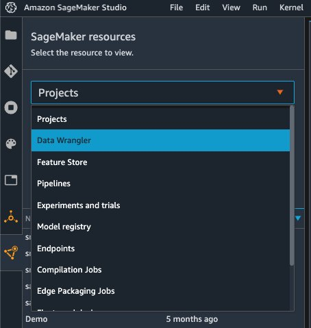\n\n#### **Import data**\n\nTo import your data, complete the following steps:\n\n1. Choose **[Amazon S3](https://aws.amazon.com/cn/s3/?trk=cndc-detail)** and locate the patients.csv file in the S3 bucket.\n2. In the **Details** pane, choose **First K** for **Sampling**.\n3. Enter ```1100``` for **Sample size**.\n In the preview pane, Data Wrangler pulls the first 100 rows from the dataset and lists them as a preview.\n4. Choose **Import**.\n Data Wrangler selects the first 1,100 patients from the total patients (11,000 rows) generated by Synthea and imports the data. The sampling approach lets Data Wrangler only process the sample data. It enables us to develop our data flow with a smaller dataset, which results in quicker processing and a shorter feedback loop. After we create the data flow, we can submit the developed recipe to a [SageMaker processing](https://docs.aws.amazon.com/sagemaker/latest/dg/processing-job.html) job to horizontally scale out the processing for the full or larger dataset in a distributed fashion.\n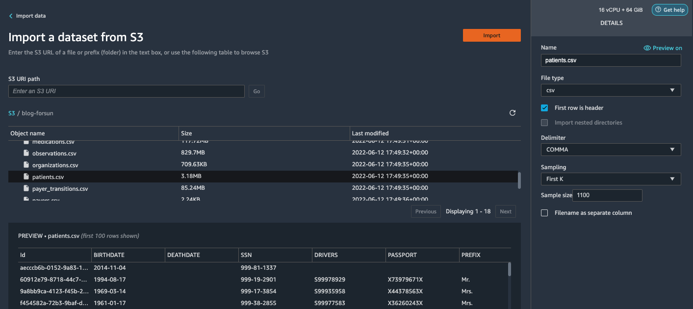\n5. Repeat this process for the ```conditions``` and ```observations``` datasets.\na. For the ```conditions``` dataset, enter ```37000``` for Sample size, which is 1/10 of the total 370,000 rows generated by Synthea.\nb. For the ```observations``` dataset, enter ```500000``` for Sample size, which is 1/10 of the total observations 5 million rows generated by Synthea.\n\nYou should see three datasets as shown in the following screenshot.\n\n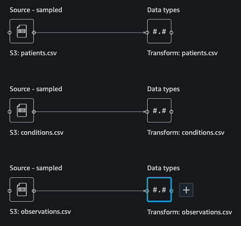\n\n#### **Transform the data**\n\nData transformation is the process of changing the structure, value, or format of one or more columns in the dataset. The process is usually developed by a data engineer and can be challenging for people with a smaller data engineering skillset to decipher the logic proposed for the transformation. Data transformation is part of the broader feature engineering process, and the correct sequence of steps is another important criterion to keep in mind while devising such recipes.\n\nData Wrangler is designed to be a low-code tool to reduce the barrier of entry for effective data preparation. It comes with over 300 preconfigured data transformations for you to choose from without writing a single line of code. In the following sections, we see how to transform the imported datasets in Data Wrangler.\n\n#### **Drop columns in patients.csv**\n\nWe first drop some columns from the ```patients``` dataset. Dropping redundant columns removes non-relevant information from the dataset and helps us reduce the amount of computing resources required to process the dataset and train a model. In this section, we drop columns such as SSN or passport number based on common sense that these columns have no predictive value. In other words, they don’t help our model predict heart failure. Our study is also not concerned about other columns such as birthplace or healthcare expenses’ influence to a patient’s heart failure, so we drop them as well. Redundant columns can also be identified by running the built-in analyses like target leakage, feature correlation, multicollinearity, and more, which are built into Data Wrangler. For more details on the supported analyses types, refer to [Analyze and Visualize](https://docs.aws.amazon.com/sagemaker/latest/dg/data-wrangler-analyses.html). Additionally, you can use the [Data Quality and Insights Report](https://docs.aws.amazon.com/sagemaker/latest/dg/data-wrangler-data-insights.html) to perform automated analyses on the datasets to arrive at a list of redundant columns to eliminate.\n\n1. Choose the plus sign next to **Data types** for the patients.csv dataset and choose **Add transform**.\n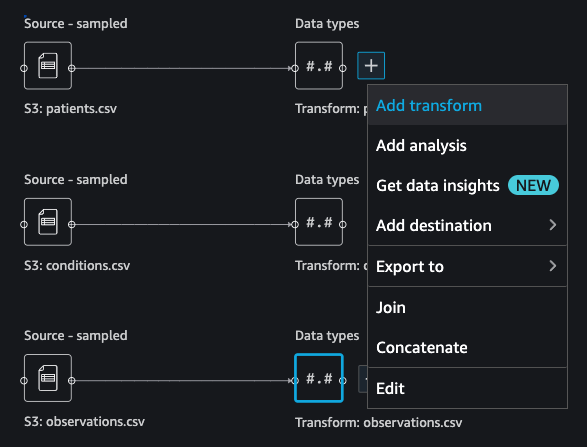\n2. Choose **Add step** and choose **Manage columns**.\n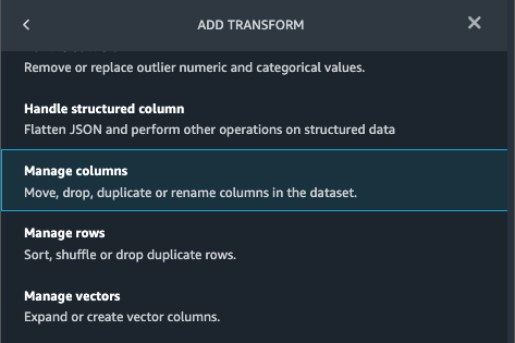\n3. For **Transform**¸ choose **Drop column**.\n4. For **Columns to drop**, choose the following columns:\n\n\ta. ```SSN```\n\tb. ```DRIVERS```\n\tc. ```PASSPORT```\n\td. ```PREFIX```\n\te. ```FIRST```\n\tf. ```LAST```\n\tg. ```SUFFIX```\n\th. ```MAIDEN```\n\ti. ```RACE```\n\tj. ```ETHNICITY```\n\tk. ```BIRTHPLACE```\n\tl. ```ADDRESS```\n\tm. ```CITY```\n\tn. ```STATE```\n\to. ```COUNTY```\n\tp. ```ZIP```\n\tq. ```LAT```\n\tr. ```LON```\n\ts. ```HEALTHCARE_EXPENSES```\n\tt. ```HEALTHCARE_COVERAGE```\n5. Choose **Preview** to review the transformed dataset, then choose **Add**.\n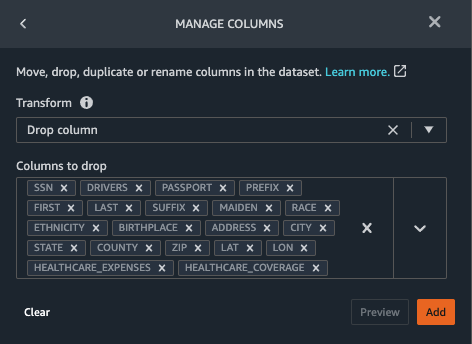\n\nYou should see the step Drop column in your list of transforms.\n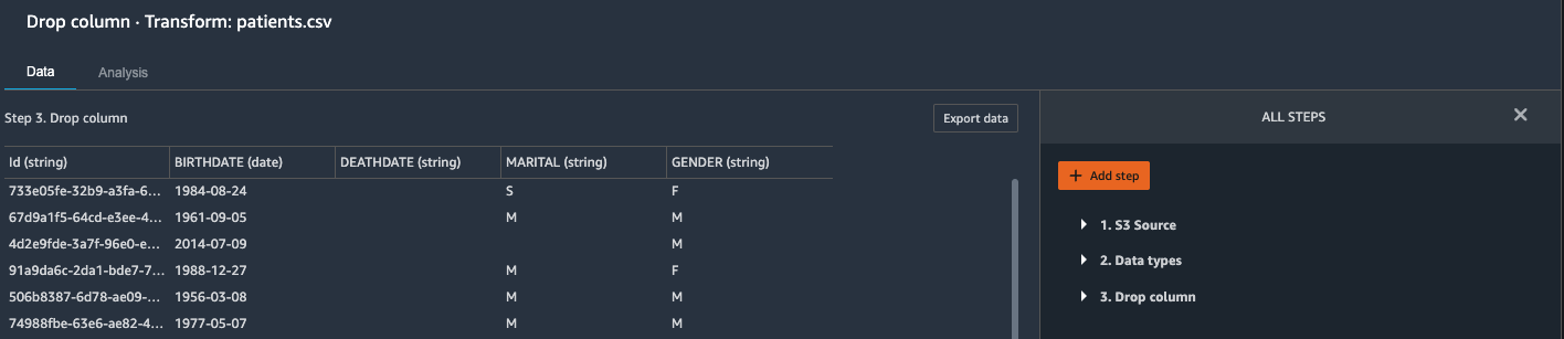\n\n#### **Featurize date/time in patients.csv**\n\nNow we use the Featurize date/time function to generate the new feature ```Year``` from the ```BIRTHDATE``` column in the ```patients``` dataset. We use the new feature in a subsequent step to calculate a patient’s age at the time of observation takes place.\n\n1. In the **Transforms** pane of your **Drop column** page for the ```patients``` dataset, choose **Add step**.\n2. Choose the **Featurize date/time** transform.\n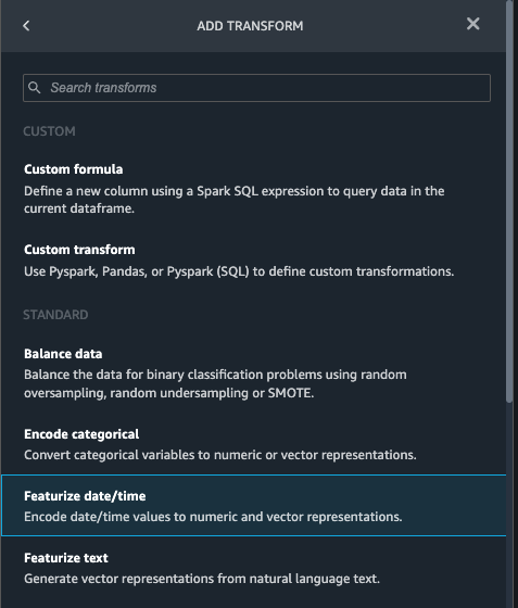\n3. Choose **Extract columns**.\n4. For **Input columns**, add the column ```BIRTHDATE```.\n5. Select **Year** and deselect **Month, Day, Hour, Minute, Second**.\n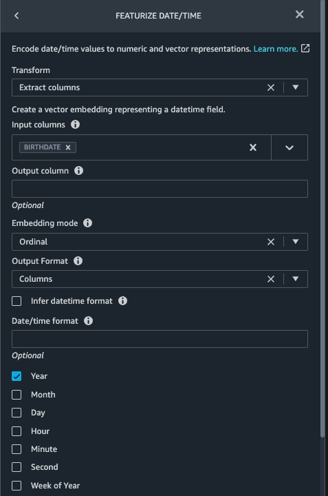\n6. Choose **Preview**, then choose **Add**.\n\n#### **Add transforms in observations.csv**\n\nData Wrangler supports custom transforms using Python (user-defined functions), PySpark, Pandas, or PySpark (SQL). You can choose your transform type based on your familiarity with each option and preference. For the latter three options, Data Wrangler exposes the variable ```df``` for you to access the dataframe and apply transformations on it. For a detailed explanation and examples, refer to [Custom Transforms](https://docs.aws.amazon.com/sagemaker/latest/dg/data-wrangler-transform.html#data-wrangler-transform-custom). In this section, we add three custom transforms to the ```observations``` dataset.\n\n1. Add a transform to observations.csv and drop the ```DESCRIPTION``` column.\n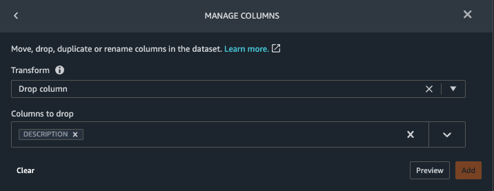\n2. Choose **Preview**, then choose **Add**.\n3. In the **Transforms** pane, choose **Add step** and choose **Custom transform**.\n4. On the drop-down menu, choose **Python (Pandas)**.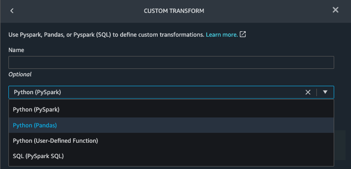\n5. Enter the following code:\n ```\\ndf = df[df[\\"CODE\\"].isin(['8867-4','8480-6','8462-4','39156-5','777-3'])]\\n```\nThese are LONIC codes that correspond to the following observations we’re interested in using as features for predicting heart failure:\n\n```\\nheart rate: 8867-4\\nsystolic blood pressure: 8480-6\\ndiastolic blood pressure: 8462-4\\nbody mass index (BMI): 39156-5\\nplatelets [#/volume] in Blood: 777-3\\n```\n\n6. Choose **Preview**, then choose **Add**.\n7. Add a transform to extract ```Year``` and ```Quarter``` from the DATE column.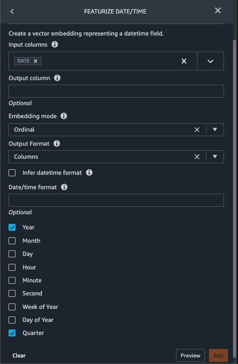\n8. Choose **Preview**, then choose **Add**.\n9. Choose **Add ste**p and choose **Custom transform**.\n10. On the drop-down menu, choose **Python (PySpark)**.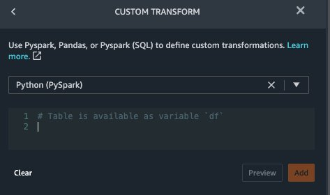The five types of observations may not always be recorded on the same date. For example, a patient may visit their family doctor on January 21 and have their systolic blood pressure, diastolic blood pressure, heart rate, and body mass index measured and recorded. However, a lab test that includes platelets may be done at a later date on February 2. Therefore, it’s not always possible to join dataframes by the observation date. Here we join dataframes on a coarse granularity at the quarter basis.\n11. Enter the following code:\n```\\nfrom pyspark.sql.functions import col\\n\\nsystolic_df = (\\n df.select(\\"patient\\", \\"DATE_year\\", \\"DATE_quarter\\", \\"value\\")\\n .withColumnRenamed(\\"value\\", \\"systolic\\")\\n .filter((col(\\"code\\") == \\"8480-6\\"))\\n )\\n\\ndiastolic_df = (\\n df.select(\\"patient\\", \\"DATE_year\\", \\"DATE_quarter\\", \\"value\\")\\n .withColumnRenamed('value', 'diastolic')\\n .filter((col(\\"code\\") == \\"8462-4\\"))\\n )\\n\\nhr_df = (\\n df.select(\\"patient\\", \\"DATE_year\\", \\"DATE_quarter\\", \\"value\\")\\n .withColumnRenamed('value', 'hr')\\n .filter((col(\\"code\\") == \\"8867-4\\"))\\n )\\n\\nbmi_df = (\\n df.select(\\"patient\\", \\"DATE_year\\", \\"DATE_quarter\\", \\"value\\")\\n .withColumnRenamed('value', 'bmi')\\n .filter((col(\\"code\\") == \\"39156-5\\"))\\n )\\n\\nplatelets_df = (\\n df.select(\\"patient\\", \\"DATE_year\\", \\"DATE_quarter\\", \\"value\\")\\n .withColumnRenamed('value', 'platelets')\\n .filter((col(\\"code\\") == \\"777-3\\"))\\n )\\n\\ndf = (\\n systolic_df.join(diastolic_df, [\\"patient\\", \\"DATE_year\\", \\"DATE_quarter\\"])\\n .join(hr_df, [\\"patient\\", \\"DATE_year\\", \\"DATE_quarter\\"])\\n .join(bmi_df, [\\"patient\\", \\"DATE_year\\", \\"DATE_quarter\\"])\\n .join(platelets_df, [\\"patient\\", \\"DATE_year\\", \\"DATE_quarter\\"])\\n)\\n```\n\n12. Choose **Preview**, then choose **Add**.\n13. Choose **Add step**, then choose **Manage rows**.\n14. For **Transform**, choose **Drop duplicates**.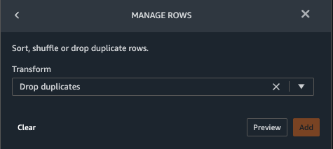\n15. Choose **Preview**, then choose **Add**.\n16. Choose **Add step** and choose **Custom transform**.\n17. On the drop-down menu, choose **Python (Pandas)**.\n18. Enter the following code to take an average of data points that share the same time value\n```\\nimport pandas as pd\\ndf.loc[:, df.columns != 'patient']=df.loc[:, df.columns != 'patient'].apply(pd.to_numeric)\\ndf = df.groupby(['patient','DATE_year','DATE_quarter']).mean().round(0).reset_index()\\n```\n19. Choose Preview, then choose Add.\n\n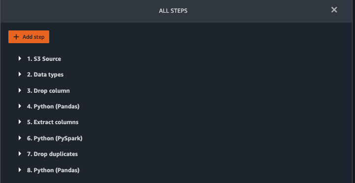\n\n#### **Join patients.csv and observations.csv**\n\nIn this step, we showcase how to effectively and easily perform complex joins on datasets without writing any code via Data Wrangler’s powerful UI. To learn more about the supported types of joins, refer to [TransformData](https://docs.amazonaws.cn/en_us/sagemaker/latest/dg/data-wrangler-transform.html).\n\n1. To the right of **Transform: patients.csv**, choose the plus sign next to **Steps** and choose **Join**.\nYou can see the transformed patients.csv file listed under Datasets in the left pane.\n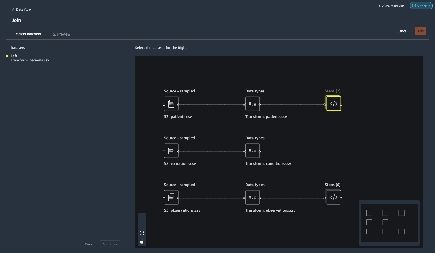\n2. To the right of Transform: observations.csv, click on the Steps to initiate the join operation.\nThe transformed observations.csv file is now listed under Datasets in the left pane.\n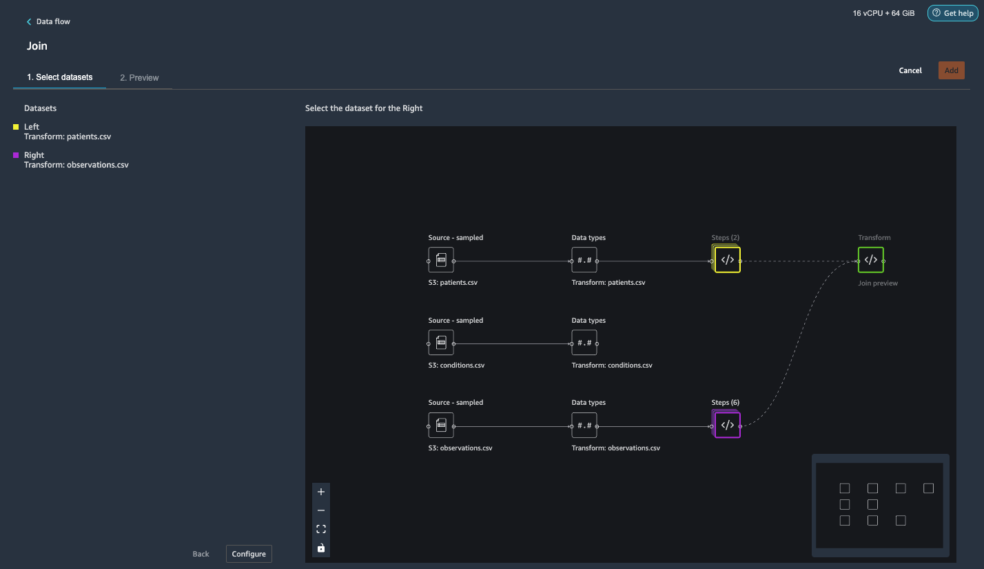\n3. Choose **Configure**.\n4. For **Join Type**, choose Inner.\n5. For **Left**, choose **Id**.\n6. For **Right**, choose **patient**.\n7. Choose **Preview**, then choose **Add**.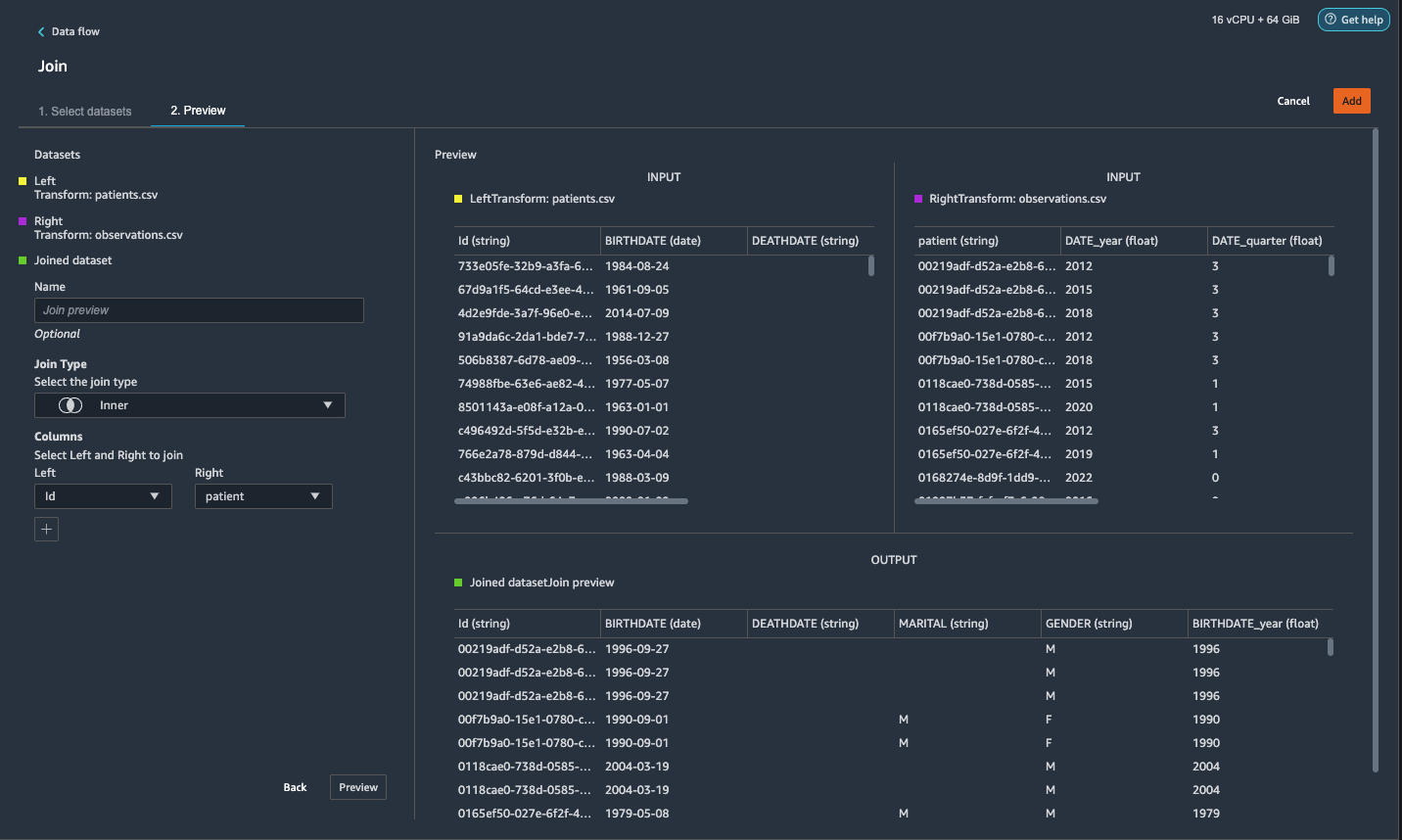\n\n#### **Add a custom transform to the joined datasets**\n\nIn this step, we calculate a patient’s age at the time of observation. We also drop columns that are no longer needed.\n\n1. Choose the plus sign next to **1st Join** and choose **Add transform**.\n2. Add a custom transform in Pandas:\n```\\ndf['age'] = df['DATE_year'] - df['BIRTHDATE_year']\\ndf = df.drop(columns=['BIRTHDATE','DEATHDATE','BIRTHDATE_year','patient'])\\n```\n\n3. Choose **Preview**, then choose **Add**.\n\n#### **Add custom transforms to conditions.csv**\n\n1. Choose the plus sign next to **Transform: conditions.csv** and choose **Add transform**.\n2. Add a custom transform in Pandas:\n```\\ndf = df[df[\\"CODE\\"].isin(['84114007', '88805009', '59621000', '44054006', '53741008', '449868002', '49436004'])]\\ndf = df.drop(columns=['DESCRIPTION','ENCOUNTER','STOP'])\\n```\n\n**Note**: As we demonstrated earlier, you can drop columns either using custom code or using the built-in transformations provided by Data Wrangler. Custom transformations within Data Wrangler provides the flexibility to bring your own transformation logic in the form of code snippets in the supported frameworks. These snippets can later be searched and applied if needed.\n\nThe codes in the preceding transform are SNOMED-CT codes that correspond to the following conditions. The ```heart failure``` or ```chronic congestive heart failure``` condition becomes the label. We use the remaining conditions as features for predicting heart failure. We also drop a few columns that are no longer needed.\n\n```\\nHeart failure: 84114007\\nChronic congestive heart failure: 88805009\\nHypertension: 59621000\\nDiabetes: 44054006\\nCoronary Heart Disease: 53741008\\nSmokes tobacco daily: 449868002\\nAtrial Fibrillation: 49436004\\n```\n3. Next, let’s add a custom transform in PySpark:\n```\\ndiabetes_df = (\\n df.select(\\"patient\\", \\"start\\")\\n .withColumnRenamed(\\"start\\", \\"diabetes\\")\\n .filter((col(\\"code\\") == \\"44054006\\"))\\n )\\n\\ncoronary_df = (\\n df.select(\\"patient\\", \\"start\\")\\n .withColumnRenamed(\\"start\\", \\"coronary\\")\\n .filter((col(\\"code\\") == \\"53741008\\"))\\n )\\n\\nsmoke_df = (\\n df.select(\\"patient\\", \\"start\\")\\n .withColumnRenamed(\\"start\\", \\"smoke\\")\\n .filter((col(\\"code\\") == \\"449868002\\"))\\n )\\n\\natrial_df = (\\n df.select(\\"patient\\", \\"start\\")\\n .withColumnRenamed(\\"start\\", \\"atrial\\")\\n .filter((col(\\"code\\") == \\"49436004\\"))\\n )\\n\\ndf = (\\n heartfailure_df.join(hypertension_df, [\\"patient\\"], \\"leftouter\\").withColumn(\\"has_hypertension\\", when(col(\\"hypertension\\") < col(\\"heartfailure\\"), 1).otherwise(0))\\n .join(diabetes_df, [\\"patient\\"], \\"leftouter\\").withColumn(\\"has_diabetes\\", when(col(\\"diabetes\\") < col(\\"heartfailure\\"), 1).otherwise(0))\\n .join(coronary_df, [\\"patient\\"], \\"leftouter\\").withColumn(\\"has_coronary\\", when(col(\\"coronary\\") < col(\\"heartfailure\\"), 1).otherwise(0))\\n .join(smoke_df, [\\"patient\\"], \\"leftouter\\").withColumn(\\"has_smoke\\", when(col(\\"smoke\\") < col(\\"heartfailure\\"), 1).otherwise(0))\\n .join(atrial_df, [\\"patient\\"], \\"leftouter\\").withColumn(\\"has_atrial\\", when(col(\\"atrial\\") < col(\\"heartfailure\\"), 1).otherwise(0))\\n)\\n```\nWe perform a left outer join to keep all entries in the heart failure dataframe. A new column ```has_xxx``` is calculated for each condition other than heart failure based on the condition’s start date. We’re only interested in medical conditions that were recorded prior to the heart failure and use them as features for predicting heart failure.\n\n4. Add a built-in Manage columns transform to drop the redundant columns that are no longer needed:\n\n\n\ta. ```hypertension```\n\tb. ```diabetes```\n\tc. ```coronary```\n\td. ```smoke```\n\te. ```atrial```\n5. Extract Year and Quarter from the heartfailure column.\nThis matches the granularity we used earlier in the transformation of the observations dataset.\n6. We should have a total of 6 steps for conditions.csv.\n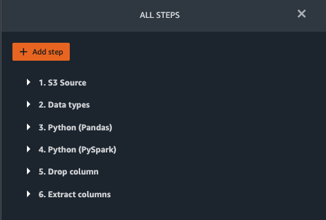\n\n#### **Join conditions.csv to the joined dataset**\n\nWe now perform a new join to join the conditions dataset to the joined ```patients``` and ```observations``` dataset.\n\n1. Choose **Transform: 1st Join**.\n2. Choose the plus sign and choose **Join**.\n3. Choose **Steps** next to **Transform: conditions.csv**.\n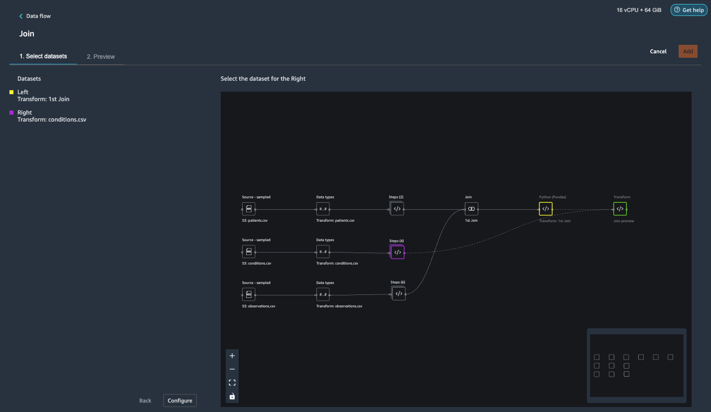\n4. Choose **Configure**.\n5. For **Join Type**, choose **Left outer**.\n6. For Left, choose Id.\n7. For **Right**, choose **patient**.\n8. Choose **Preview**, then choose **Add**.\n\n#### **Add transforms to the joined datasets**\n\nNow that we have all three datasets joined, let’s apply some additional transformations.\n\n","render":"<p>Machine learning (ML) is disrupting a lot of industries at an unprecedented pace. The healthcare and life sciences (HCLS) industry has been going through a rapid evolution in recent years embracing ML across a multitude of use cases for delivering quality care and improving patient outcomes.</p>\n<p>In a typical ML lifecycle, data engineers and scientists spend the majority of their time on the data preparation and feature engineering steps before even getting started with the process of model building and training. Having a tool that can lower the barrier to entry for data preparation, thereby improving productivity, is a highly desirable ask for these personas. <a href=\\"https://docs.aws.amazon.com/sagemaker/latest/dg/data-wrangler.html\\" target=\\"_blank\\">Amazon SageMaker Data Wrangler</a> is purpose built by AWS to reduce the learning curve and enable data practitioners to accomplish data preparation, cleaning, and feature engineering tasks in less effort and time. It offers a GUI interface with many built-in functions and integrations with other AWS services such as <a href=\\"https://aws.amazon.com/cn/s3/\\" target=\\"_blank\\">Amazon Simple Storage Service</a> ([Amazon S3](https://aws.amazon.com/cn/s3/?trk=cndc-detail)) and <a href=\\"https://aws.amazon.com/cn/sagemaker/feature-store/\\" target=\\"_blank\\">Amazon SageMaker Feature Store</a>, as well as partner data sources including Snowflake and Databricks.</p>\\n<p>In this post, we demonstrate how to use Data Wrangler to prepare healthcare data for training a model to predict heart failure, given a patient’s demographics, prior medical conditions, and lab test result history.</p>\n<h4><a id=\\"Solution_overview_6\\"></a><strong>Solution overview</strong></h4>\\n<p>The solution consists of the following steps:</p>\n<ol>\\n<li>Acquire a healthcare dataset as input to Data Wrangler.</li>\n<li>Use Data Wrangler’s built-in transformation functions to transform the dataset. This includes drop columns, featurize data/time, join datasets, impute missing values, encode categorical variables, scale numeric values, balance the dataset, and more.</li>\n<li>Use Data Wrangler’s custom transform function (Pandas or PySpark code) to supplement additional transformations required beyond the built-in transformations and demonstrate the extensibility of Data Wrangler. This includes filter rows, group data, form new dataframes based on conditions, and more.</li>\n<li>Use Data Wrangler’s built-in visualization functions to perform visual analysis. This includes target leakage, feature correlation, quick model, and more.</li>\n<li>Use Data Wrangler’s built-in export options to export the transformed dataset to Amazon S3.</li>\n<li>Launch a Jupyter notebook to use the transformed dataset in Amazon S3 as input to train a model.</li>\n</ol>\\n<h4><a id=\\"Generate_a_dataset_17\\"></a><strong>Generate a dataset</strong></h4>\\n<p>Now that we have settled on the ML problem statement, we first set our sights on acquiring the data we need. Research studies such as <a href=\\"https://www.kaggle.com/datasets/andrewmvd/heart-failure-clinical-data\\" target=\\"_blank\\">Heart Failure Prediction</a> may provide data that’s already in good shape. However, we often encounter scenarios where the data is quite messy and requires joining, cleansing, and several other transformations that are very specific to the healthcare domain before it can be used for ML training. We want to find or generate data that is messy enough and walk you through the steps of preparing it using Data Wrangler. With that in mind, we picked Synthea as a tool to generate synthetic data that fits our goal. <a href=\\"https://github.com/synthetichealth/synthea\\" target=\\"_blank\\">Synthea</a> is an open-source synthetic patient generator that models the medical history of synthetic patients. To generate your dataset, complete the following steps:</p>\\n<ol>\\n<li>\\n<p>Follow the instructions as per the <a href=\\"https://docs.aws.amazon.com/sagemaker/latest/dg/onboard-quick-start.html\\" target=\\"_blank\\">quick start</a> documentation to create an <a href=\\"https://aws.amazon.com/cn/sagemaker/studio/\\" target=\\"_blank\\">Amazon SageMaker Studio</a> domain and launch Studio.<br />\\nThis is a prerequisite step. It is optional if Studio is already set up in your account.</p>\n</li>\\n<li>\\n<p>After Studio is launched, on the <strong>Launcher</strong> tab, choose <strong>System terminal</strong>.<br />\\nThis launches a terminal session that gives you a command line interface to work with.<br />\\n<img src=\\"https://dev-media.amazoncloud.cn/19c9a0b4fe874d3091535a331aa0fe42_image.png\\" alt=\\"image.png\\" /></p>\n</li>\\n<li>\\n<p>To install Synthea and generate the dataset in CSV format, run the following commands in the launched terminal session:</p>\n</li>\\n</ol>\n<pre><code class=\\"lang-\\">\$ sudo yum install -y java-1.8.0-openjdk-devel\\n\$ export JAVA_HOME=/usr/lib/jvm/jre-1.8.0-openjdk.x86_64\\n\$ export PATH=\$JAVA_HOME/bin:\$PATH\\n\$ git clone https://github.com/synthetichealth/synthea\\n\$ git checkout v3.0.0\\n\$ cd synthea\\n\$ ./run_synthea --exporter.csv.export=true -p 10000\\n</code></pre>\\n<p>We supply a parameter to generate the datasets with a population size of 10,000. Note the size parameter denotes the number of alive members of the population. Additionally, Synthea also generates data for dead members of the population which might add a few extra data points on top of the specified sample size.</p>\n<p>Wait until the data generation is complete. This step usually takes around an hour or less. Synthea generates multiple datasets, including <code>patients</code>, <code>medications</code>, <code>allergies</code>, <code>conditions</code>, and more. For this post, we use three of the resulting datasets:</p>\\n<ul>\\n<li><strong>patients.csv</strong> – This dataset is about 3.2 MB and contains approximately 11,000 rows of patient data (25 columns including patient ID, birthdate, gender, address, and more)</li>\\n<li><strong>conditions.csv</strong> – This dataset is about 47 MB and contains approximately 370,000 rows of medical condition data (six columns including patient ID, condition start date, condition code, and more)</li>\\n<li><strong>observations.csv</strong> – This dataset is about 830 MB and contains approximately 5 million rows of observation data (eight columns including patient ID, observation date, observation code, value, and more)</li>\\n</ul>\n<p>There is a one-to-many relationship between the <code>patients</code> and <code>conditions</code> datasets. There is also a one-to-many relationship between the <code>patients</code> and <code>observations</code> datasets. For a detailed data dictionary, refer to <a href=\\"https://github.com/synthetichealth/synthea/wiki/CSV-File-Data-Dictionary\\" target=\\"_blank\\">CSV File Data Dictionary</a>.</p>\\n<ol start=\\"4\\">\\n<li>To upload the generated datasets to a source bucket in Amazon S3, run the following commands in the terminal session:</li>\n</ol>\\n<pre><code class=\\"lang-\\">\$ cd ./output/csv\\n\$ aws s3 sync . s3://&lt;source bucket name&gt;/\\n</code></pre>\\n<h4><a id=\\"Launch_Data_Wrangler_55\\"></a><strong>Launch Data Wrangler</strong></h4>\\n<p>Choose <strong>SageMaker resources</strong> in the navigation page in Studio and on the <strong>Projects</strong> menu, choose <strong>Data Wrangler</strong> tocreate a Data Wrangler data flow. For detailed steps how to launch Data Wrangler from within Studio, refer to <a href=\\"https://docs.aws.amazon.com/sagemaker/latest/dg/data-wrangler-getting-started.html\\" target=\\"_blank\\">Get Started with Data Wrangler</a>.</p>\\n<p><img src=\\"https://dev-media.amazoncloud.cn/674ea00289154e948ef847d2de0f18cf_image.png\\" alt=\\"image.png\\" /></p>\n<h4><a id=\\"Import_data_61\\"></a><strong>Import data</strong></h4>\\n<p>To import your data, complete the following steps:</p>\n<ol>\\n<li>Choose <strong>Amazon S3</strong> and locate the patients.csv file in the S3 bucket.</li>\\n<li>In the <strong>Details</strong> pane, choose <strong>First K</strong> for <strong>Sampling</strong>.</li>\\n<li>Enter <code>1100</code> for <strong>Sample size</strong>.<br />\\nIn the preview pane, Data Wrangler pulls the first 100 rows from the dataset and lists them as a preview.</li>\n<li>Choose <strong>Import</strong>.<br />\\nData Wrangler selects the first 1,100 patients from the total patients (11,000 rows) generated by Synthea and imports the data. The sampling approach lets Data Wrangler only process the sample data. It enables us to develop our data flow with a smaller dataset, which results in quicker processing and a shorter feedback loop. After we create the data flow, we can submit the developed recipe to a <a href=\\"https://docs.aws.amazon.com/sagemaker/latest/dg/processing-job.html\\" target=\\"_blank\\">SageMaker processing</a> job to horizontally scale out the processing for the full or larger dataset in a distributed fashion.<br />\\n<img src=\\"https://dev-media.amazoncloud.cn/611f41f7a5514204bbdbc5d74b3dfd71_image.png\\" alt=\\"image.png\\" /></li>\n<li>Repeat this process for the <code>conditions</code> and <code>observations</code> datasets.<br />\\na. For the <code>conditions</code> dataset, enter <code>37000</code> for Sample size, which is 1/10 of the total 370,000 rows generated by Synthea.<br />\\nb. For the <code>observations</code> dataset, enter <code>500000</code> for Sample size, which is 1/10 of the total observations 5 million rows generated by Synthea.</li>\\n</ol>\n<p>You should see three datasets as shown in the following screenshot.</p>\n<p><img src=\\"https://dev-media.amazoncloud.cn/3dbfa639a0804afbad9c8f574ca970fc_image.png\\" alt=\\"image.png\\" /></p>\n<h4><a id=\\"Transform_the_data_80\\"></a><strong>Transform the data</strong></h4>\\n<p>Data transformation is the process of changing the structure, value, or format of one or more columns in the dataset. The process is usually developed by a data engineer and can be challenging for people with a smaller data engineering skillset to decipher the logic proposed for the transformation. Data transformation is part of the broader feature engineering process, and the correct sequence of steps is another important criterion to keep in mind while devising such recipes.</p>\n<p>Data Wrangler is designed to be a low-code tool to reduce the barrier of entry for effective data preparation. It comes with over 300 preconfigured data transformations for you to choose from without writing a single line of code. In the following sections, we see how to transform the imported datasets in Data Wrangler.</p>\n<h4><a id=\\"Drop_columns_in_patientscsv_86\\"></a><strong>Drop columns in patients.csv</strong></h4>\\n<p>We first drop some columns from the <code>patients</code> dataset. Dropping redundant columns removes non-relevant information from the dataset and helps us reduce the amount of computing resources required to process the dataset and train a model. In this section, we drop columns such as SSN or passport number based on common sense that these columns have no predictive value. In other words, they don’t help our model predict heart failure. Our study is also not concerned about other columns such as birthplace or healthcare expenses’ influence to a patient’s heart failure, so we drop them as well. Redundant columns can also be identified by running the built-in analyses like target leakage, feature correlation, multicollinearity, and more, which are built into Data Wrangler. For more details on the supported analyses types, refer to <a href=\\"https://docs.aws.amazon.com/sagemaker/latest/dg/data-wrangler-analyses.html\\" target=\\"_blank\\">Analyze and Visualize</a>. Additionally, you can use the <a href=\\"https://docs.aws.amazon.com/sagemaker/latest/dg/data-wrangler-data-insights.html\\" target=\\"_blank\\">Data Quality and Insights Report</a> to perform automated analyses on the datasets to arrive at a list of redundant columns to eliminate.</p>\\n<ol>\\n<li>\\n<p>Choose the plus sign next to <strong>Data types</strong> for the patients.csv dataset and choose <strong>Add transform</strong>.<br />\\n<img src=\\"https://dev-media.amazoncloud.cn/562d09d3612b421a9efa274b79e99838_image.png\\" alt=\\"image.png\\" /></p>\n</li>\\n<li>\\n<p>Choose <strong>Add step</strong> and choose <strong>Manage columns</strong>.<br />\\n<img src=\\"https://dev-media.amazoncloud.cn/1891f3bb69d948ce804f45ba7e1a149b_image.png\\" alt=\\"image.png\\" /></p>\n</li>\\n<li>\\n<p>For <strong>Transform</strong>¸ choose <strong>Drop column</strong>.</p>\\n</li>\n<li>\\n<p>For <strong>Columns to drop</strong>, choose the following columns:</p>\\n<p>a. <code>SSN</code><br />\\nb. <code>DRIVERS</code><br />\\nc. <code>PASSPORT</code><br />\\nd. <code>PREFIX</code><br />\\ne. <code>FIRST</code><br />\\nf. <code>LAST</code><br />\\ng. <code>SUFFIX</code><br />\\nh. <code>MAIDEN</code><br />\\ni. <code>RACE</code><br />\\nj. <code>ETHNICITY</code><br />\\nk. <code>BIRTHPLACE</code><br />\\nl. <code>ADDRESS</code><br />\\nm. <code>CITY</code><br />\\nn. <code>STATE</code><br />\\no. <code>COUNTY</code><br />\\np. <code>ZIP</code><br />\\nq. <code>LAT</code><br />\\nr. <code>LON</code><br />\\ns. <code>HEALTHCARE_EXPENSES</code><br />\\nt. <code>HEALTHCARE_COVERAGE</code></p>\\n</li>\n<li>\\n<p>Choose <strong>Preview</strong> to review the transformed dataset, then choose <strong>Add</strong>.<br />\\n<img src=\\"https://dev-media.amazoncloud.cn/313f9232e2ad4e788a0a449b45e5da8b_image.png\\" alt=\\"image.png\\" /></p>\n</li>\\n</ol>\n<p>You should see the step Drop column in your list of transforms.<br />\\n<img src=\\"https://dev-media.amazoncloud.cn/efeda9d4c7424226becb2997d781e48a_image.png\\" alt=\\"image.png\\" /></p>\n<h4><a id=\\"Featurize_datetime_in_patientscsv_123\\"></a><strong>Featurize date/time in patients.csv</strong></h4>\\n<p>Now we use the Featurize date/time function to generate the new feature <code>Year</code> from the <code>BIRTHDATE</code> column in the <code>patients</code> dataset. We use the new feature in a subsequent step to calculate a patient’s age at the time of observation takes place.</p>\\n<ol>\\n<li>In the <strong>Transforms</strong> pane of your <strong>Drop column</strong> page for the <code>patients</code> dataset, choose <strong>Add step</strong>.</li>\\n<li>Choose the <strong>Featurize date/time</strong> transform.<br />\\n<img src=\\"https://dev-media.amazoncloud.cn/dbb7fad0d02848db9fcd6c937ca3b47b_image.png\\" alt=\\"image.png\\" /></li>\n<li>Choose <strong>Extract columns</strong>.</li>\\n<li>For <strong>Input columns</strong>, add the column <code>BIRTHDATE</code>.</li>\\n<li>Select <strong>Year</strong> and deselect <strong>Month, Day, Hour, Minute, Second</strong>.<br />\\n<img src=\\"https://dev-media.amazoncloud.cn/497cb754981949628f819bff38c5ab8c_image.png\\" alt=\\"image.png\\" /></li>\n<li>Choose <strong>Preview</strong>, then choose <strong>Add</strong>.</li>\\n</ol>\n<h4><a id=\\"Add_transforms_in_observationscsv_136\\"></a><strong>Add transforms in observations.csv</strong></h4>\\n<p>Data Wrangler supports custom transforms using Python (user-defined functions), PySpark, Pandas, or PySpark (SQL). You can choose your transform type based on your familiarity with each option and preference. For the latter three options, Data Wrangler exposes the variable <code>df</code> for you to access the dataframe and apply transformations on it. For a detailed explanation and examples, refer to <a href=\\"https://docs.aws.amazon.com/sagemaker/latest/dg/data-wrangler-transform.html#data-wrangler-transform-custom\\" target=\\"_blank\\">Custom Transforms</a>. In this section, we add three custom transforms to the <code>observations</code> dataset.</p>\\n<ol>\\n<li>Add a transform to observations.csv and drop the <code>DESCRIPTION</code> column.<br />\\n<img src=\\"https://dev-media.amazoncloud.cn/6185631c9fa64e14936a73abc9cef149_image.png\\" alt=\\"image.png\\" /></li>\n<li>Choose <strong>Preview</strong>, then choose <strong>Add</strong>.</li>\\n<li>In the <strong>Transforms</strong> pane, choose <strong>Add step</strong> and choose <strong>Custom transform</strong>.</li>\\n<li>On the drop-down menu, choose <strong>Python (Pandas)</strong>.<img src=\\"https://dev-media.amazoncloud.cn/ebb0d274b06247deacb153d69d531b49_image.png\\" alt=\\"image.png\\" /></li>\n<li>Enter the following code:</li>\n</ol>\\n<pre><code class=\\"lang-\\">df = df[df[&quot;CODE&quot;].isin(['8867-4','8480-6','8462-4','39156-5','777-3'])]\\n</code></pre>\\n<p>These are LONIC codes that correspond to the following observations we’re interested in using as features for predicting heart failure:</p>\n<pre><code class=\\"lang-\\">heart rate: 8867-4\\nsystolic blood pressure: 8480-6\\ndiastolic blood pressure: 8462-4\\nbody mass index (BMI): 39156-5\\nplatelets [#/volume] in Blood: 777-3\\n</code></pre>\\n<ol start=\\"6\\">\\n<li>Choose <strong>Preview</strong>, then choose <strong>Add</strong>.</li>\\n<li>Add a transform to extract <code>Year</code> and <code>Quarter</code> from the DATE column.<img src=\\"https://dev-media.amazoncloud.cn/19bd77057429473db2eafaa13ef7225e_image.png\\" alt=\\"image.png\\" /></li>\n<li>Choose <strong>Preview</strong>, then choose <strong>Add</strong>.</li>\\n<li>Choose <strong>Add ste</strong>p and choose <strong>Custom transform</strong>.</li>\\n<li>On the drop-down menu, choose <strong>Python (PySpark)</strong>.<img src=\\"https://dev-media.amazoncloud.cn/9a0e2745f3904dc5a3d8f55d200b807d_image.png\\" alt=\\"image.png\\" />The five types of observations may not always be recorded on the same date. For example, a patient may visit their family doctor on January 21 and have their systolic blood pressure, diastolic blood pressure, heart rate, and body mass index measured and recorded. However, a lab test that includes platelets may be done at a later date on February 2. Therefore, it’s not always possible to join dataframes by the observation date. Here we join dataframes on a coarse granularity at the quarter basis.</li>\n<li>Enter the following code:</li>\n</ol>\\n<pre><code class=\\"lang-\\">from pyspark.sql.functions import col\\n\\nsystolic_df = (\\n df.select(&quot;patient&quot;, &quot;DATE_year&quot;, &quot;DATE_quarter&quot;, &quot;value&quot;)\\n .withColumnRenamed(&quot;value&quot;, &quot;systolic&quot;)\\n .filter((col(&quot;code&quot;) == &quot;8480-6&quot;))\\n )\\n\\ndiastolic_df = (\\n df.select(&quot;patient&quot;, &quot;DATE_year&quot;, &quot;DATE_quarter&quot;, &quot;value&quot;)\\n .withColumnRenamed('value', 'diastolic')\\n .filter((col(&quot;code&quot;) == &quot;8462-4&quot;))\\n )\\n\\nhr_df = (\\n df.select(&quot;patient&quot;, &quot;DATE_year&quot;, &quot;DATE_quarter&quot;, &quot;value&quot;)\\n .withColumnRenamed('value', 'hr')\\n .filter((col(&quot;code&quot;) == &quot;8867-4&quot;))\\n )\\n\\nbmi_df = (\\n df.select(&quot;patient&quot;, &quot;DATE_year&quot;, &quot;DATE_quarter&quot;, &quot;value&quot;)\\n .withColumnRenamed('value', 'bmi')\\n .filter((col(&quot;code&quot;) == &quot;39156-5&quot;))\\n )\\n\\nplatelets_df = (\\n df.select(&quot;patient&quot;, &quot;DATE_year&quot;, &quot;DATE_quarter&quot;, &quot;value&quot;)\\n .withColumnRenamed('value', 'platelets')\\n .filter((col(&quot;code&quot;) == &quot;777-3&quot;))\\n )\\n\\ndf = (\\n systolic_df.join(diastolic_df, [&quot;patient&quot;, &quot;DATE_year&quot;, &quot;DATE_quarter&quot;])\\n .join(hr_df, [&quot;patient&quot;, &quot;DATE_year&quot;, &quot;DATE_quarter&quot;])\\n .join(bmi_df, [&quot;patient&quot;, &quot;DATE_year&quot;, &quot;DATE_quarter&quot;])\\n .join(platelets_df, [&quot;patient&quot;, &quot;DATE_year&quot;, &quot;DATE_quarter&quot;])\\n)\\n</code></pre>\\n<ol start=\\"12\\">\\n<li>Choose <strong>Preview</strong>, then choose <strong>Add</strong>.</li>\\n<li>Choose <strong>Add step</strong>, then choose <strong>Manage rows</strong>.</li>\\n<li>For <strong>Transform</strong>, choose <strong>Drop duplicates</strong>.<img src=\\"https://dev-media.amazoncloud.cn/8dfa19d8106f4b8a98d0e678ea250a55_image.png\\" alt=\\"image.png\\" /></li>\n<li>Choose <strong>Preview</strong>, then choose <strong>Add</strong>.</li>\\n<li>Choose <strong>Add step</strong> and choose <strong>Custom transform</strong>.</li>\\n<li>On the drop-down menu, choose <strong>Python (Pandas)</strong>.</li>\\n<li>Enter the following code to take an average of data points that share the same time value</li>\n</ol>\\n<pre><code class=\\"lang-\\">import pandas as pd\\ndf.loc[:, df.columns != 'patient']=df.loc[:, df.columns != 'patient'].apply(pd.to_numeric)\\ndf = df.groupby(['patient','DATE_year','DATE_quarter']).mean().round(0).reset_index()\\n</code></pre>\\n<ol start=\\"19\\">\\n<li>Choose Preview, then choose Add.</li>\n</ol>\\n<p><img src=\\"https://dev-media.amazoncloud.cn/b42026d068714a39b0dce9eb5ddcbf41_image.png\\" alt=\\"image.png\\" /></p>\n<h4><a id=\\"Join_patientscsv_and_observationscsv_222\\"></a><strong>Join patients.csv and observations.csv</strong></h4>\\n<p>In this step, we showcase how to effectively and easily perform complex joins on datasets without writing any code via Data Wrangler’s powerful UI. To learn more about the supported types of joins, refer to <a href=\\"https://docs.amazonaws.cn/en_us/sagemaker/latest/dg/data-wrangler-transform.html\\" target=\\"_blank\\">TransformData</a>.</p>\\n<ol>\\n<li>To the right of <strong>Transform: patients.csv</strong>, choose the plus sign next to <strong>Steps</strong> and choose <strong>Join</strong>.<br />\\nYou can see the transformed patients.csv file listed under Datasets in the left pane.<br />\\n<img src=\\"https://dev-media.amazoncloud.cn/aae3b029270941f39dda2ae375d19101_image.png\\" alt=\\"image.png\\" /></li>\n<li>To the right of Transform: observations.csv, click on the Steps to initiate the join operation.<br />\\nThe transformed observations.csv file is now listed under Datasets in the left pane.<br />\\n<img src=\\"https://dev-media.amazoncloud.cn/4e13fef6324d45f689af8c07c1ef313e_image.png\\" alt=\\"image.png\\" /></li>\n<li>Choose <strong>Configure</strong>.</li>\\n<li>For <strong>Join Type</strong>, choose Inner.</li>\\n<li>For <strong>Left</strong>, choose <strong>Id</strong>.</li>\\n<li>For <strong>Right</strong>, choose <strong>patient</strong>.</li>\\n<li>Choose <strong>Preview</strong>, then choose <strong>Add</strong>.<img src=\\"https://dev-media.amazoncloud.cn/c480e572c5b74876a97a76d837a759bc_image.png\\" alt=\\"image.png\\" /></li>\n</ol>\\n<h4><a id=\\"Add_a_custom_transform_to_the_joined_datasets_238\\"></a><strong>Add a custom transform to the joined datasets</strong></h4>\\n<p>In this step, we calculate a patient’s age at the time of observation. We also drop columns that are no longer needed.</p>\n<ol>\\n<li>Choose the plus sign next to <strong>1st Join</strong> and choose <strong>Add transform</strong>.</li>\\n<li>Add a custom transform in Pandas:</li>\n</ol>\\n<pre><code class=\\"lang-\\">df['age'] = df['DATE_year'] - df['BIRTHDATE_year']\\ndf = df.drop(columns=['BIRTHDATE','DEATHDATE','BIRTHDATE_year','patient'])\\n</code></pre>\\n<ol start=\\"3\\">\\n<li>Choose <strong>Preview</strong>, then choose <strong>Add</strong>.</li>\\n</ol>\n<h4><a id=\\"Add_custom_transforms_to_conditionscsv_251\\"></a><strong>Add custom transforms to conditions.csv</strong></h4>\\n<ol>\\n<li>Choose the plus sign next to <strong>Transform: conditions.csv</strong> and choose <strong>Add transform</strong>.</li>\\n<li>Add a custom transform in Pandas:</li>\n</ol>\\n<pre><code class=\\"lang-\\">df = df[df[&quot;CODE&quot;].isin(['84114007', '88805009', '59621000', '44054006', '53741008', '449868002', '49436004'])]\\ndf = df.drop(columns=['DESCRIPTION','ENCOUNTER','STOP'])\\n</code></pre>\\n<p><strong>Note</strong>: As we demonstrated earlier, you can drop columns either using custom code or using the built-in transformations provided by Data Wrangler. Custom transformations within Data Wrangler provides the flexibility to bring your own transformation logic in the form of code snippets in the supported frameworks. These snippets can later be searched and applied if needed.</p>\\n<p>The codes in the preceding transform are SNOMED-CT codes that correspond to the following conditions. The <code>heart failure</code> or <code>chronic congestive heart failure</code> condition becomes the label. We use the remaining conditions as features for predicting heart failure. We also drop a few columns that are no longer needed.</p>\\n<pre><code class=\\"lang-\\">Heart failure: 84114007\\nChronic congestive heart failure: 88805009\\nHypertension: 59621000\\nDiabetes: 44054006\\nCoronary Heart Disease: 53741008\\nSmokes tobacco daily: 449868002\\nAtrial Fibrillation: 49436004\\n</code></pre>\\n<ol start=\\"3\\">\\n<li>Next, let’s add a custom transform in PySpark:</li>\n</ol>\\n<pre><code class=\\"lang-\\">diabetes_df = (\\n df.select(&quot;patient&quot;, &quot;start&quot;)\\n .withColumnRenamed(&quot;start&quot;, &quot;diabetes&quot;)\\n .filter((col(&quot;code&quot;) == &quot;44054006&quot;))\\n )\\n\\ncoronary_df = (\\n df.select(&quot;patient&quot;, &quot;start&quot;)\\n .withColumnRenamed(&quot;start&quot;, &quot;coronary&quot;)\\n .filter((col(&quot;code&quot;) == &quot;53741008&quot;))\\n )\\n\\nsmoke_df = (\\n df.select(&quot;patient&quot;, &quot;start&quot;)\\n .withColumnRenamed(&quot;start&quot;, &quot;smoke&quot;)\\n .filter((col(&quot;code&quot;) == &quot;449868002&quot;))\\n )\\n\\natrial_df = (\\n df.select(&quot;patient&quot;, &quot;start&quot;)\\n .withColumnRenamed(&quot;start&quot;, &quot;atrial&quot;)\\n .filter((col(&quot;code&quot;) == &quot;49436004&quot;))\\n )\\n\\ndf = (\\n heartfailure_df.join(hypertension_df, [&quot;patient&quot;], &quot;leftouter&quot;).withColumn(&quot;has_hypertension&quot;, when(col(&quot;hypertension&quot;) &lt; col(&quot;heartfailure&quot;), 1).otherwise(0))\\n .join(diabetes_df, [&quot;patient&quot;], &quot;leftouter&quot;).withColumn(&quot;has_diabetes&quot;, when(col(&quot;diabetes&quot;) &lt; col(&quot;heartfailure&quot;), 1).otherwise(0))\\n .join(coronary_df, [&quot;patient&quot;], &quot;leftouter&quot;).withColumn(&quot;has_coronary&quot;, when(col(&quot;coronary&quot;) &lt; col(&quot;heartfailure&quot;), 1).otherwise(0))\\n .join(smoke_df, [&quot;patient&quot;], &quot;leftouter&quot;).withColumn(&quot;has_smoke&quot;, when(col(&quot;smoke&quot;) &lt; col(&quot;heartfailure&quot;), 1).otherwise(0))\\n .join(atrial_df, [&quot;patient&quot;], &quot;leftouter&quot;).withColumn(&quot;has_atrial&quot;, when(col(&quot;atrial&quot;) &lt; col(&quot;heartfailure&quot;), 1).otherwise(0))\\n)\\n</code></pre>\\n<p>We perform a left outer join to keep all entries in the heart failure dataframe. A new column <code>has_xxx</code> is calculated for each condition other than heart failure based on the condition’s start date. We’re only interested in medical conditions that were recorded prior to the heart failure and use them as features for predicting heart failure.</p>\\n<ol start=\\"4\\">\\n<li>\\n<p>Add a built-in Manage columns transform to drop the redundant columns that are no longer needed:</p>\n<p>a. <code>hypertension</code><br />\\nb. <code>diabetes</code><br />\\nc. <code>coronary</code><br />\\nd. <code>smoke</code><br />\\ne. <code>atrial</code></p>\\n</li>\n<li>\\n<p>Extract Year and Quarter from the heartfailure column.<br />\\nThis matches the granularity we used earlier in the transformation of the observations dataset.</p>\n</li>\\n<li>\\n<p>We should have a total of 6 steps for conditions.csv.<br />\\n<img src=\\"https://dev-media.amazoncloud.cn/e4a403ac17764614b620bcc5eb408a2c_image.png\\" alt=\\"image.png\\" /></p>\n</li>\\n</ol>\n<h4><a id=\\"Join_conditionscsv_to_the_joined_dataset_322\\"></a><strong>Join conditions.csv to the joined dataset</strong></h4>\\n<p>We now perform a new join to join the conditions dataset to the joined <code>patients</code> and <code>observations</code> dataset.</p>\\n<ol>\\n<li>Choose <strong>Transform: 1st Join</strong>.</li>\\n<li>Choose the plus sign and choose <strong>Join</strong>.</li>\\n<li>Choose <strong>Steps</strong> next to <strong>Transform: conditions.csv</strong>.<br />\\n<img src=\\"https://dev-media.amazoncloud.cn/0d80ac48e025442386009a2c3b01697b_image.png\\" alt=\\"image.png\\" /></li>\n<li>Choose <strong>Configure</strong>.</li>\\n<li>For <strong>Join Type</strong>, choose <strong>Left outer</strong>.</li>\\n<li>For Left, choose Id.</li>\n<li>For <strong>Right</strong>, choose <strong>patient</strong>.</li>\\n<li>Choose <strong>Preview</strong>, then choose <strong>Add</strong>.<img src=\\"https://dev-media.amazoncloud.cn/e1fc4ffa93d4412ea82a9ac58f3c34f7_image.png\\" alt=\\"image.png\\" /></li>\n</ol>\\n<h4><a id=\\"Add_transforms_to_the_joined_datasets_336\\"></a><strong>Add transforms to the joined datasets</strong></h4>\\n<p>Now that we have all three datasets joined, let’s apply some additional transformations.</p>\n"}