A serverless operational data lake for retail with Amazon Glue, Amazon Kinesis Data Streams, Amazon DynamoDB, and Amazon QuickSight

{"value":"Do you want to reduce stockouts at stores? Do you want to improve order delivery timelines? Do you want to provide your customers with accurate product availability, down to the millisecond? A retail operational data lake can help you transform the customer experience by providing deeper insights into a variety of operational aspects of your supply chain.\n\nIn this post, we demonstrate how to create a serverless operational data lake using AWS services, including [AWS Glue](https://aws.amazon.com/glue), Amazon Kinesis Data Streams, [Amazon DynamoDB](https://aws.amazon.com/dynamodb/), [Amazon Athena](https://aws.amazon.com/athena/), and [Amazon QuickSight](https://aws.amazon.com/quicksight).\n\nRetail operations is a critical functional area that gives retailers a competitive edge. An efficient retail operation can optimize the supply chain for a better customer experience and cost reduction. An optimized retail operation can reduce frequent stockouts and delayed shipments, and provide accurate inventory and order details. Today, a retailer’s channels aren’t just store and web—they include mobile apps, chatbots, connected devices, and social media channels. The data is both structured and unstructured. This coupled with multiple fulfillment options like buy online and pick up at store, ship from store, or ship from distribution centers, which increases the complexity of retail operations.\n\nMost retailers use a centralized order management system (OMS) for managing orders, inventory, shipments, payments, and other operational aspects. These legacy OMSs are unable to scale in response to the rapid changes in retail business models. The enterprise applications that are key for efficient and smooth retail operations rely on a central OMS. Applications for ecommerce, warehouse management, call centers, and mobile all require an OMS to get order status, inventory positions of different items, shipment status, and more. Another challenge with legacy OMSs is they’re not designed to handle unstructured data like weather data and IoT data that could impact inventory and order fulfillment. A legacy OMS that can’t scale prohibits you from implementing new business models that could transform your customer experience.\n\nA data lake is a centralized repository that allows you to store all your structured and unstructured data at any scale. An operational data lake addresses this challenge by providing easy access to structured and unstructured operational data in real time from various enterprise systems. You can store your data as is, without having to first structure the data, and run different types of analytics—from dashboards and visualizations to big data processing, real-time analytics, and machine learning (ML)—to guide better decisions. This can ease the burden on OMSs that can instead focus on order orchestration and management.\n\n#### **Solution overview**\nIn this post, we create an end-to-end pipeline to ingest, store, process, analyze, and visualize operational data like orders, inventory, and shipment updates. We use the following AWS services as key components:\n\n- Kinesis Data Streams to ingest all operational data in real time from various systems\n- DynamoDB, [Amazon Aurora](https://aws.amazon.com/rds/aurora/), and [Amazon Simple Storage Service](http://aws.amazon.com/s3) (Amazon S3) to store the data\n- [AWS Glue DataBrew](https://aws.amazon.com/glue/features/databrew/) to clean and transform the data\n- AWS Glue crawlers to catalog the data\n- Athena to query the processed data\n- A QuickSight dashboard that provides insights into various operational metrics\n\nThe following diagram illustrates the solution architecture.\n\n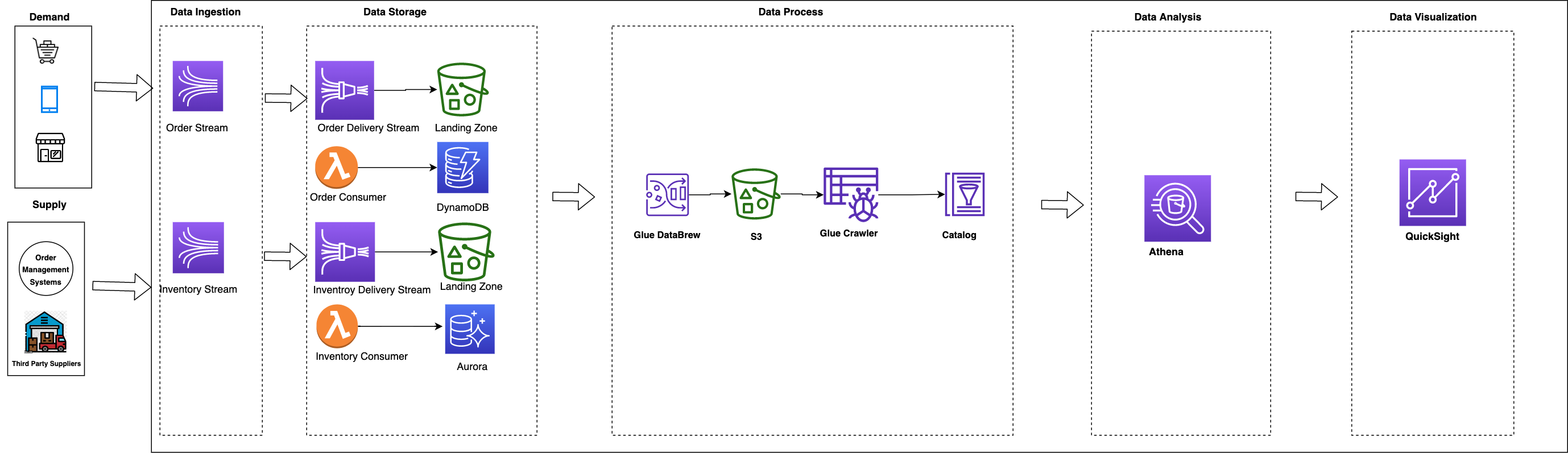\n\nThe data pipeline consists of stages to ingest, store, process, analyze, and finally visualize the data, which we discuss in more detail in the following sections.\n\n#### **Data ingestion**\nOrders and inventory data is ingested in real time from multiple sources like web applications, mobile apps, and connected devices into Kinesis Data Streams. Kinesis Data Streams is a massively scalable and durable real-time data streaming service. Kinesis Data Streams can continuously capture gigabytes of data per second from hundreds of thousands of sources, such as web applications, database events, inventory transactions, and payment transactions. Frontend systems like ecommerce applications and mobile apps ingest the order data as soon as items are added to a cart or an order is created. The OMS ingests orders when the order status changes. OMSs, stores, and third-party suppliers ingest inventory updates into the data stream.\n\nTo simulate orders, an [AWS Lambda](http://aws.amazon.com/lambda) function is triggered by a scheduled [Amazon CloudWatch](http://aws.amazon.com/cloudwatch) event every minute to ingest orders to a data stream. This function simulates the typical order management system lifecycle (order created, scheduled, released, shipped, and delivered). Similarly, a second Lambda function is triggered by a CloudWatch event to generate inventory updates. This function simulates different inventory updates such as purchase orders created from systems like the OMS or third-party suppliers. In a production environment, this data would come from frontend applications and a centralized order management system.\n\n#### **Data storage**\nThere are two types of data: hot and cold data. Hot data is consumed by frontend applications like web applications, mobile apps, and connected devices. The following are some example use cases for hot data:\n\n- When a customer is browsing products, the real-time availability of the item must be displayed\n- Customers interacting with Alexa to know the status of the order\n- A call center agent interacting with a customer needs to know the status of the customer order or its shipment details\n\nThe systems, APIs, and devices that consume this data need the data within seconds or milliseconds of the transactions.\n\nCold data is used for long-term analytics like orders over a period of time, orders by channel, top 10 items by number of orders, or planned vs. available inventory by item, warehouse, or store.\n\nFor this solution, we store orders hot data in DynamoDB. DynamoDB is a fully managed NoSQL database that delivers single-digit millisecond performance at any scale. A Lambda function processes records in the Kinesis data stream and stores it in a DynamoDB table.\n\nInventory hot data is stored in an [Amazon Aurora MySQL-Compatible Edition](https://aws.amazon.com/rds/aurora/mysql-features/) database. Inventory is transactional data that requires high consistency so that customers aren’t over-promised or under-promised when they place orders. Aurora MySQL is fully managed database that is up to five times faster than standard MySQL databases and three times faster than standard PostgreSQL databases. It provides the security, availability, and reliability of commercial databases at a tenth of the cost.\n\nAmazon S3 is object storage built to store and retrieve any amount of data from anywhere. It’s a simple storage service that offers industry-leading durability, availability, performance, security, and virtually unlimited scalability at very low cost. Order and inventory cold data is stored in Amazon S3.\n\n[Amazon Kinesis Data](https://aws.amazon.com/kinesis/data-firehose/) Firehose reads the data from the Kinesis data stream and stores it in Amazon S3. Kinesis Data Firehose is the easiest way to load streaming data into data stores and analytics tools. It can capture, transform, and load streaming data into Amazon S3, [Amazon Redshift](http://aws.amazon.com/redshift), [Amazon OpenSearch Service](https://aws.amazon.com/opensearch-service/), and Splunk, enabling near-real-time analytics.\n\n**Data processing**\nThe data processing stage involves cleaning, preparing, and transforming the data to help downstream analytics applications easily query the data. Each frontend system might have a different data format. In the data processing stage, data is cleaned and converted into a common canonical form.\n\nFor this solution, we use DataBrew to clean and convert orders into a common canonical form. DataBrew is a visual data preparation tool that makes it easy for data analysts and data scientists to prepare data with an interactive, point-and-click visual interface without writing code. DataBrew provides over 250 built-in transformations to combine, pivot, and transpose the data without writing code. The cleaning and transformation steps in DataBrew are called recipes. A scheduled DataBrew job applies the recipes to the data in an S3 bucket and stores the output in a different bucket.\n\nAWS Glue crawlers can access data stores, extract metadata, and create table definitions in the AWS Glue Data Catalog. You can schedule a crawler to crawl the transformed data and create or update the Data Catalog. The AWS Glue Data Catalog is your persistent metadata store. It’s a managed service that lets you store, annotate, and share metadata in the AWS Cloud in the same way you would in an Apache Hive metastore. We use crawlers to populate the Data Catalog with tables.\n\n**Data analysis**\nWe can query orders and inventory data from S3 buckets using Athena. Athena is an interactive query service that makes it easy to analyze data in Amazon S3 using standard SQL. Athena is serverless, so there is no infrastructure to manage, and you pay only for the queries that you run. Views are created in Athena that can be consumed by business intelligence (BI) services like QuickSight.\n\n**Data visualization**\nWe generate dashboards using QuickSight. QuickSight is a scalable, serverless, embeddable BI service powered by ML and built for the cloud. QuickSight lets you easily create and publish interactive BI dashboards that include ML-powered insights.\n\nQuickSight also has features to forecast orders, detect anomalies in the order, and provide ML-powered insights. We can create analyses such as orders over a period of time, orders split by channel, top 10 locations for orders, or order fulfillment timelines (the time it took from order creation to order delivery).\n\n#### **Walkthrough overview**\nTo implement this solution, you complete the following high-level steps:\n\n1. Create solution resources using [AWS CloudFormation](http://aws.amazon.com/cloudformation).\n2. Connect to the inventory database.\n3. Load the inventory database with tables.\n4. Create a [VPC endpoint](https://docs.aws.amazon.com/vpc/latest/privatelink/vpc-endpoints.html) using [Amazon Virtual Private Cloud](http://aws.amazon.com/vpc) (Amazon VPC).\n5. Create [gateway endpoints](https://docs.aws.amazon.com/vpc/latest/privatelink/vpce-gateway.html) for Amazon S3 on the default VPC.\n6. Enable CloudWatch rules via [Amazon EventBridge](https://aws.amazon.com/eventbridge/) to ingest the data.\n7. Transform the data using AWS Glue.\n8. Visualize the data with QuickSight.\n\n#### **Prerequisites**\nComplete the following prerequisite steps:\n\n1. Create AWS account if you don’t have done already.\n2. [Sign up for QuickSight](https://docs.aws.amazon.com/quicksight/latest/user/signing-up.html) if you’ve never used QuickSight in this account before. To use the forecast ability in QuickSight, sign up for the Enterprise Edition.\n\n#### **Create resources with AWS CloudFormation**\nTo launch the provided CloudFormation template, complete the following steps:\n\n1. Choose **Launch Stack**:\n[](https://console.aws.amazon.com/cloudformation/home?region=us-east-1#/stacks/create/template?stackName=operational-data-lake&templateURL=https://aws-blogs-artifacts-public.s3.amazonaws.com/artifacts/BDB-1266/Datalake_Blog_CF.yaml)\n2. Choose **Next**.\n3. For **Stack name**, enter a name.\n4. Provide the following parameters:\n\t- The name of the S3 bucket that holds all the data for the data lake.The\n\t- name of the database that holds the inventory tables.\n\t- The database user name.\n\t- The database password.\n5. Enter any tags you want to assign to the stack and choose **Next**.\n6. Select the acknowledgement check boxes and choose **Create stack**.\n\nThe stack takes 5–10 minutes to complete.\n\nOn the AWS CloudFormation console, you can navigate to the stack’s **Outputs** tab to review the resources you created.\n\n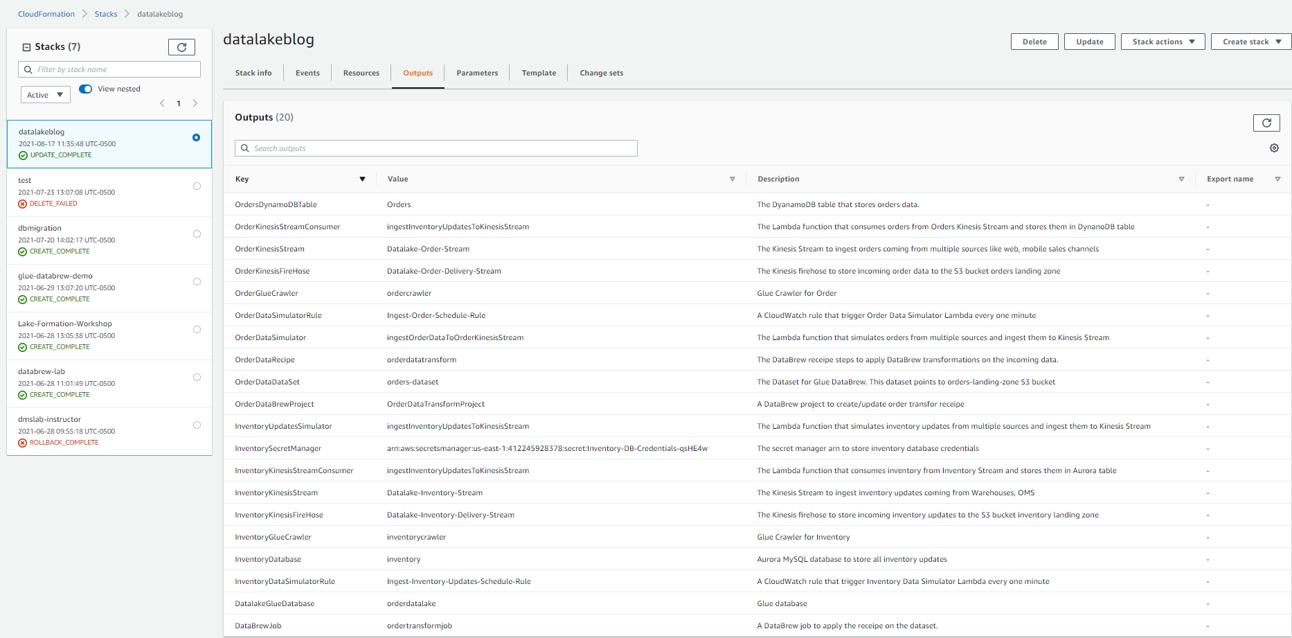\n\nIf you open the S3 bucket you created, you can observe its folder structure. The stack creates sample order data for the last 7 days.\n\n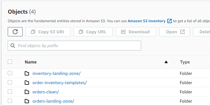\n\n#### **Connect to the inventory database**\nTo connect to your database in the query editor, complete the following steps:\n\n1. On the Amazon RDS console, choose the Region you deployed the stack in.\n\n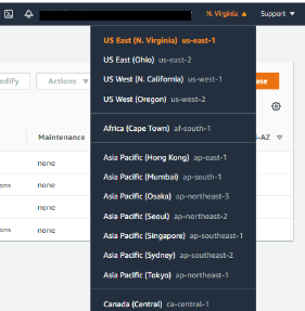\n\n2. In the navigation pane, choose **Query Editor**.\n\n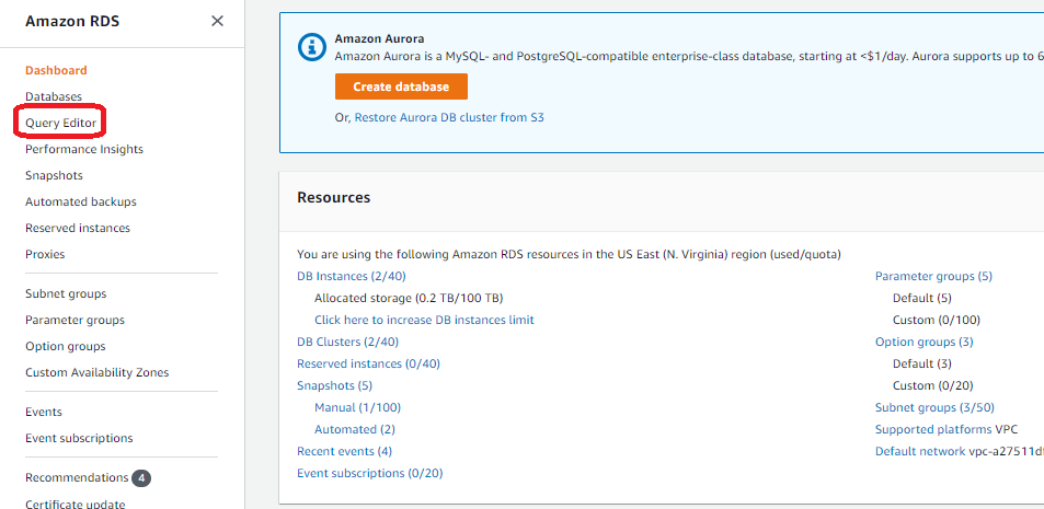\n\nIf you haven’t connected to this database before, the **Connect to database** page opens.\n\n3. For **Database instance** or cluster, choose your database.\n4. For **Database username**, choose **Connect with a Secrets Manager ARN**.\nThe database user name and password provided during stack creation are stored in AWS Secrets Manager. Alternatively, you can choose Add new database credentials and enter the database user name and password you provided when creating the stack.\n5. For **Secrets Manager ARN**, enter the value for the key ```InventorySecretManager``` from the CloudFormation stack outputs.\n6. Optionally, enter the name of your database.\n7. Choose **Connect to database**.\n\n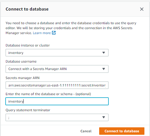\n\n\n#### **Load the inventory database with tables**\nEnter the following DDL statement in the query editor and choose **Run**:\n\n```\nCREATE TABLE INVENTORY (\n ItemID varchar(25) NOT NULL,\n ShipNode varchar(25) NOT NULL,\n SupplyType varchar(25) NOT NULL,\n SupplyDemandType varchar(25) NOT NULL,\n ItemName varchar(25),\n UOM varchar(10),\n Quantity int(11) NOT NULL,\n ETA varchar(25)\t ,\n UpdatedDate DATE,\n PRIMARY KEY (ItemID,ShipNode,SupplyType)\n);\n```\n\n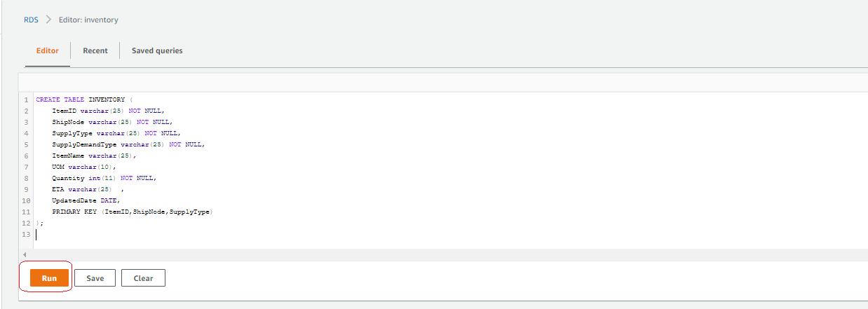\n\n#### **Create a VPC endpoint**\nTo create your VPC endpoint, complete the following steps:\n\n1. On the Amazon VPC console, choose **VPC Dashboard**.\n2. Choose **Endpoints** in the navigation pane.\n3. Choose **Create Endpoint**.\n\n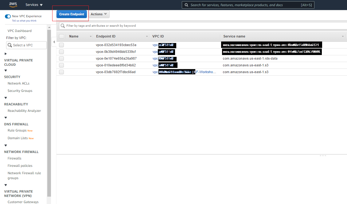\n\n4. For **Service category**, select **AWS services**.\n5. For **Service name**, search for ```rds``` and choose the service name ending with ```rds-data```.\n6. For **VPC**, choose **the default VPC**.\n\n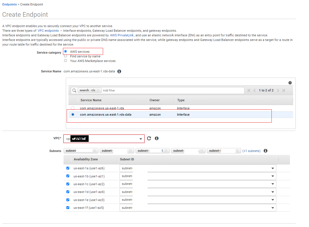\n\n7. Leave the remaining settings at their default and choose **Create endpoint**.\n\n#### **Create a gateway endpoint for Amazon S3**\nTo create your gateway endpoint, complete the following steps:\n\n1. On the Amazon VPC console, choose **VPC Dashboard**.\n2. Choose **Endpoints** in the navigation pane.\n3. Choose **Create Endpoint**.\n4. For **Service category**, select **AWS services**.\n\t1. For **Service name**, search for ```S3``` and choose the service name with type **Gateway**.\n6. For **VPC**, choose the default VPC.\n7. For **Configure route tables**, select the default route table.\n\n\n\n8. Leave the remaining settings at their default and choose **Create endpoint**.\n\nWait for both the gateway endpoint and VPC endpoint status to change to ```Available```.\n\n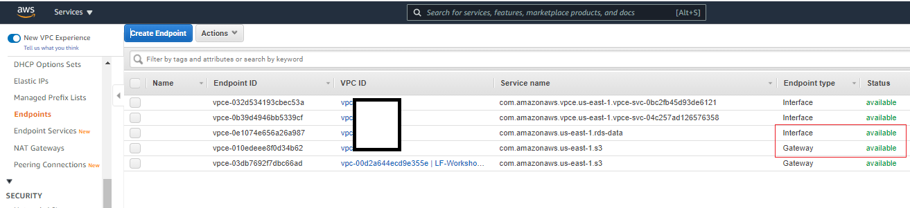\n\n#### **Enable CloudWatch rules to ingest the data**\nWe created two CloudWatch rules via the CloudFormation template to ingest the order and inventory data to Kinesis Data Streams. To enable the rules via EventBridge, complete the following steps:\n\n1. On the CloudWatch console, under **Events** in the navigation pane, choose **Rules**.\n2. Make sure you’re in the Region where you created the stack.\n3. Choose **Go to Amazon EventBridge**.\n\n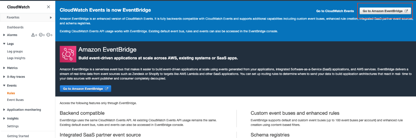\n\n4. Select the rule ```Ingest-Inventory-Update-Schedule-Rule``` and choose **Enable**.\n5. Select the rule ```Ingest-Order-Schedule-Rule``` and choose **Enable**.\n\n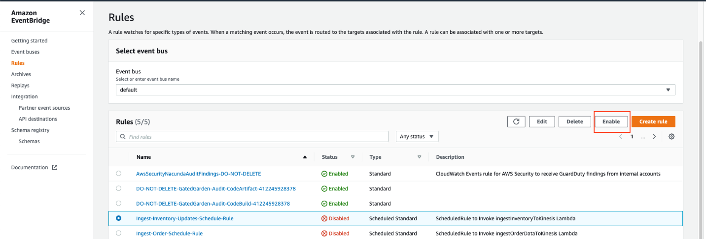\n\nAfter 5–10 minutes, the Lambda functions start ingesting orders and inventory updates to their respective streams. You can check the S3 buckets ```orders-landing-zone``` and ```inventory-landing-zone``` to confirm that the data is being populated.\n\n#### **Perform data transformation**\nOur CloudFormation stack included a DataBrew project, a DataBrew job that runs every 5 minutes, and two AWS Glue crawlers. To perform data transformation using our AWS Glue resources, complete the following steps:\n\n1. On the DataBrew console, choose **Projects** in the navigation pane.\n2. Choose the project ```OrderDataTransform```.\n\n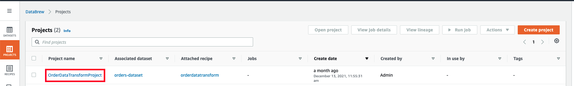\n\nYou can review the project and its recipe on this page.\n\n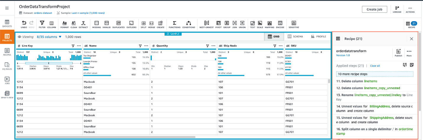\n\n3. In the navigation pane, choose **Jobs**.\n4. Review the job status to confirm it’s complete.\n\n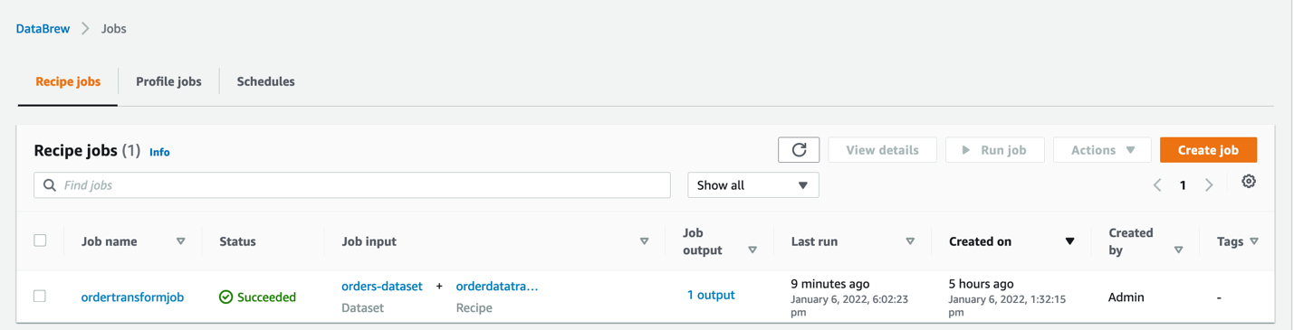\n\n5. On the AWS Glue console, choose **Crawlers** in the navigation pane.\nThe crawlers crawl the transformed data and update the Data Catalog.\n6. Review the status of the two crawlers, which run every 15 minutes.\n\n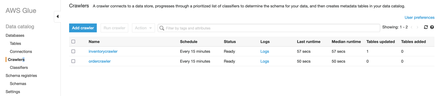\n\n7. Choose **Tables** in the navigation pane to view the two tables the crawlers created.\nIf you don’t see these tables, you can run the crawlers manually to create them.\n\n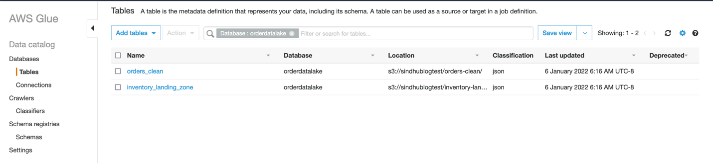\n\nYou can query the data in the tables with Athena.\n8. On the Athena console, choose **Query editor**.\nIf you haven’t created a query result location, you’re prompted to do that first.\n9. Choose **View settings** or choose the **Settings tab**.\n\n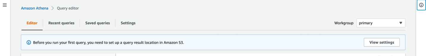\n\n10. Choose **Manage**.\n\n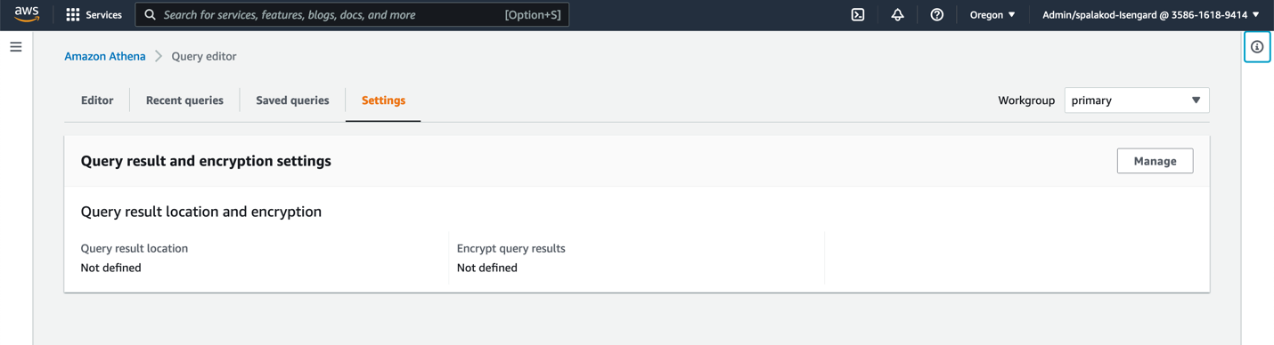\n\n11. Select the S3 bucket to store the results and choose **Choose**.\n\n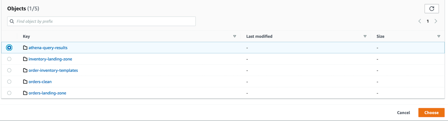\n\n12. Choose **Query editor** in the navigation pane.\n\n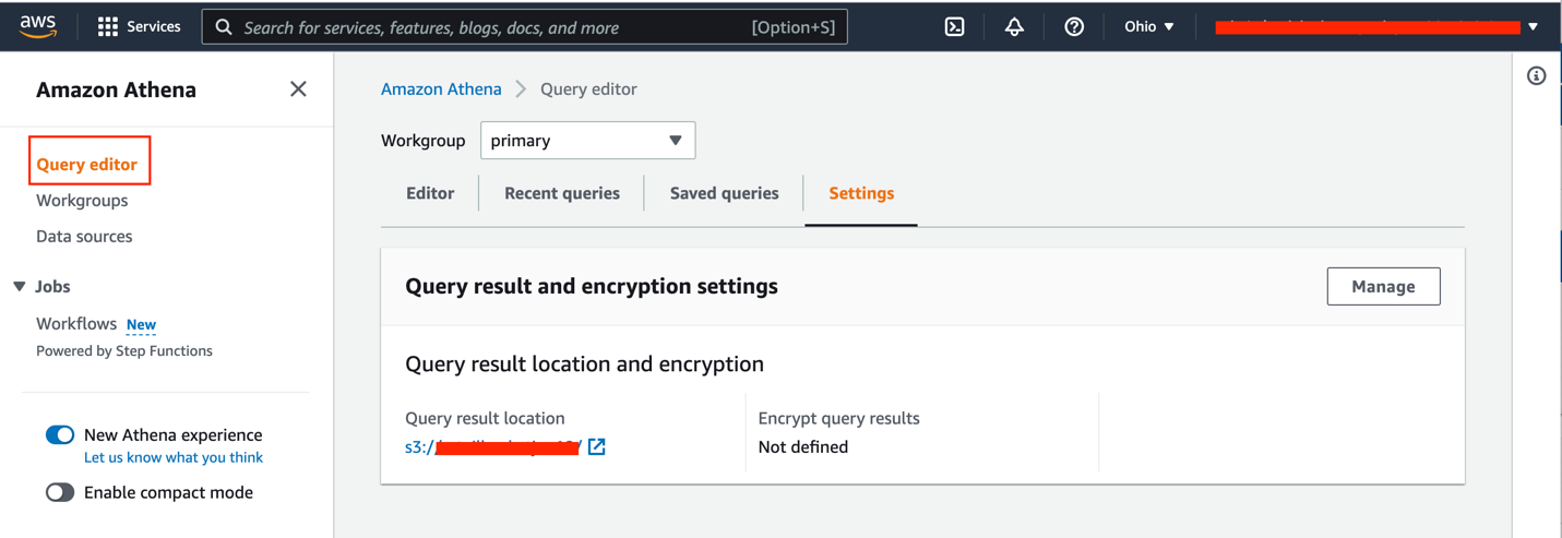\n\n13.Choose either table (right-click) and choose **Preview Table** to view the table contents.\n\n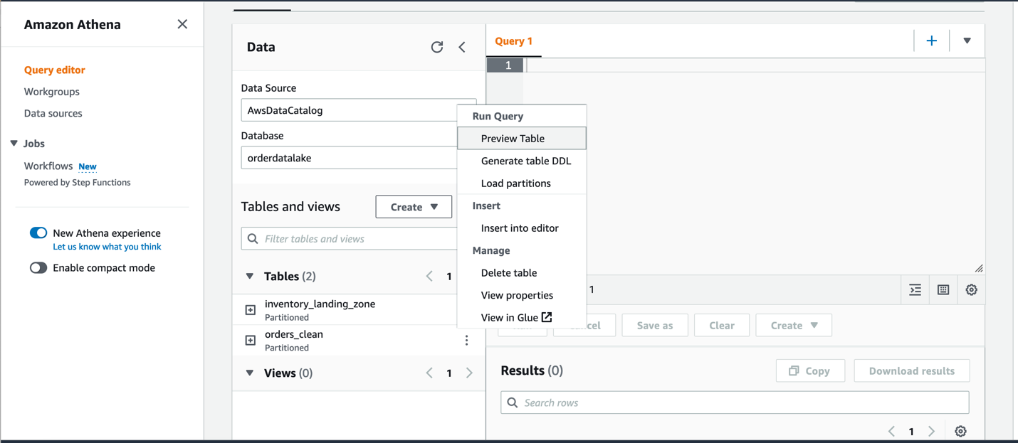\n\n#### **Visualize the data**\nIf you have never used QuickSight in this account before, complete the prerequisite step to sign up for QuickSight. To use the ML capabilities of QuickSight (such as [forecasting](https://docs.aws.amazon.com/quicksight/latest/user/forecasts-and-whatifs.html)) sign up for the Enterprise Edition using the steps in this [documentation](https://docs.aws.amazon.com/quicksight/latest/user/signing-up.html).\n\nWhile signing up for QuickSight, make sure to use the **same region** where you created the CloudFormation stack.\n\n##### **Grant QuickSight permissions**\nTo visualize your data, you must first grant relevant permissions to QuickSight to access your data.\n\n1. On the QuickSight console, on the Admin drop-down menu, choose **Manage QuickSight**.\n\n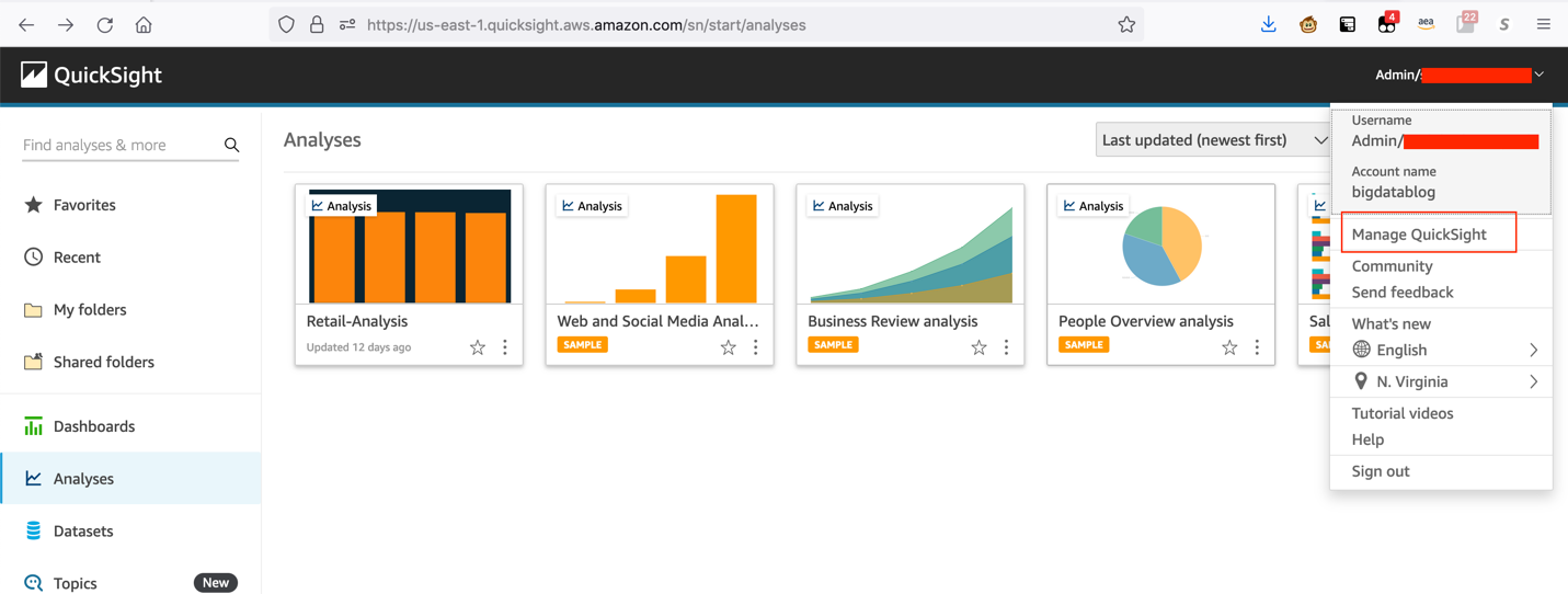\n\n2. In the navigation pane, choose **Security & permissions**.\n3. Under **QuickSight access to AWS services**, choose **Manage**.\n\n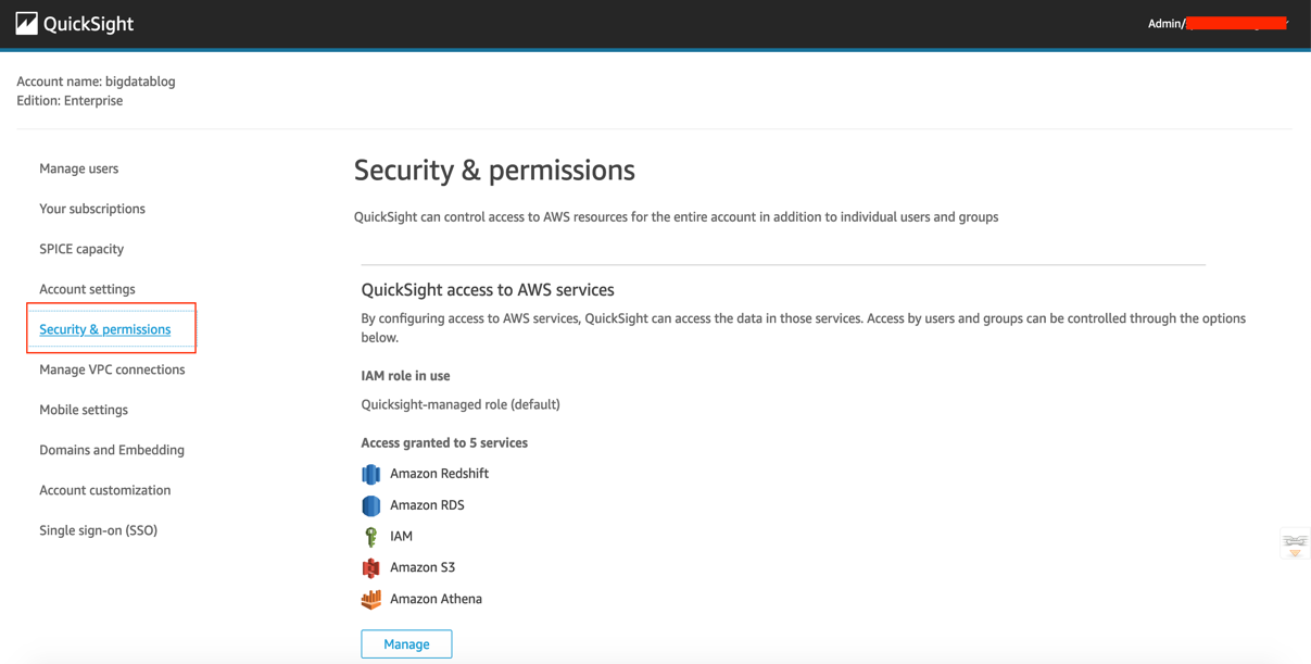\n\n4. Select **Amazon Athena**.\n5. Select **Amazon S3** to edit QuickSight access to your S3 buckets.\n6. Select the bucket you specified during stack creation (for this post, ```operational-datalake```).\n7. Choose **Finish**.\n\n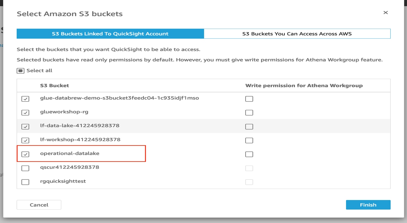\n\n8. Choose **Save**.\n\n##### **Prepare the datasets**\nTo prepare your datasets, complete the following steps:\n1. On the QuickSight console, choose **Datasets** in the navigation pane.\n2. Choose **New dataset**.\n\n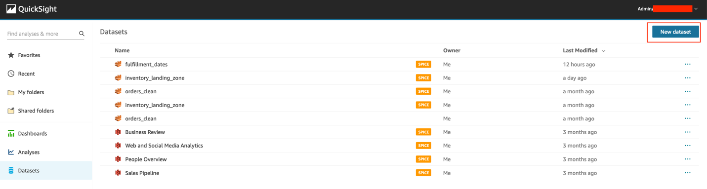\n\n3.Choose **Athena**.\n\n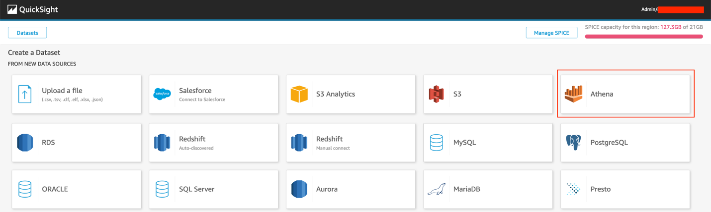\n\n4. For **Data source name**, enter ```retail-analysis```.\n5. Choose **Validate connection**.\n6. After your connection is validated, choose **Create data source**.\n\nFor Data source name, enter retail-analysis.\nChoose Validate connection.\nAfter your connection is validated, choose Create data source.\n\n7. For **Database**, choose orderdatalake.\n8. For **Tables**, select ```orders_clean```.\n9. Choose **Edit/Preview data**.\n\n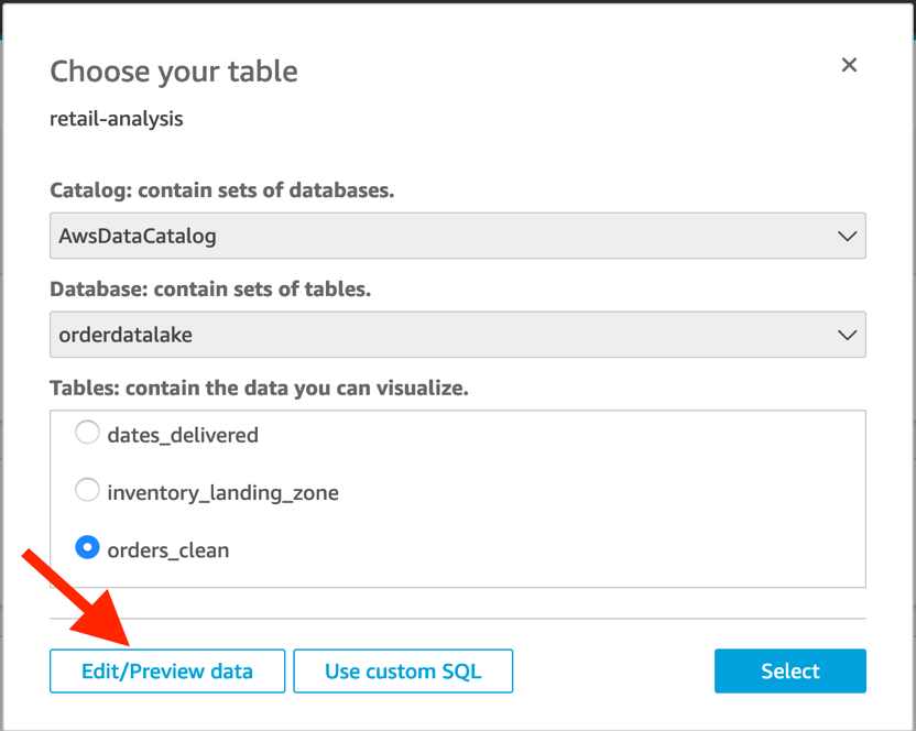\n\n10. For **Query mode**, select **SPICE**.\n[SPICE](https://docs.aws.amazon.com/quicksight/latest/user/spice.html) (Super-fast, Parallel, In-memory Calculation Engine) is the robust in-memory engine that QuickSight uses\n\n\n\n11. Choose the ```orderdatetime``` field (right-click), choose **Change data type**, and choose **Date**.\n\n\n\n12. Enter the date format as ```MM/dd/yyyy HH:mm:ss```.\n13. Choose **Validate** and **Update**.\n\n\n\n14, Change the data types of the following fields to QuickSight geospatial data types:\n\n\t- billingaddress.zipcode – Postcode\n\t- billingaddress.city – City\n\t- billingaddress.country – Country\n\t- billingaddress.state – State\n\t- shippingaddress.zipcode – Postcode\n\t- shippingaddress.city – City\n\t- shippingaddress.country – Country\n\t- shippingaddress.state – State\n15. Choose Save & publish.\n16. Choose Cancel to exit this page.\n\n\n\nLet’s create another dataset for the Athena table ```inventory_landing_zone```.\n17. Follow steps 1–7 to create a new dataset. For **Table** selection, choose inventory_landing_zone.\n18. Choose ```Edit/Preview data```.\n\n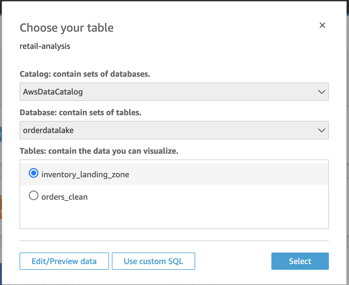\n\n19. For **Query mode**, select **SPICE**.\n20. Choose **Save & publish**.\n21. Choose **Cancel** to exit this page.\n\n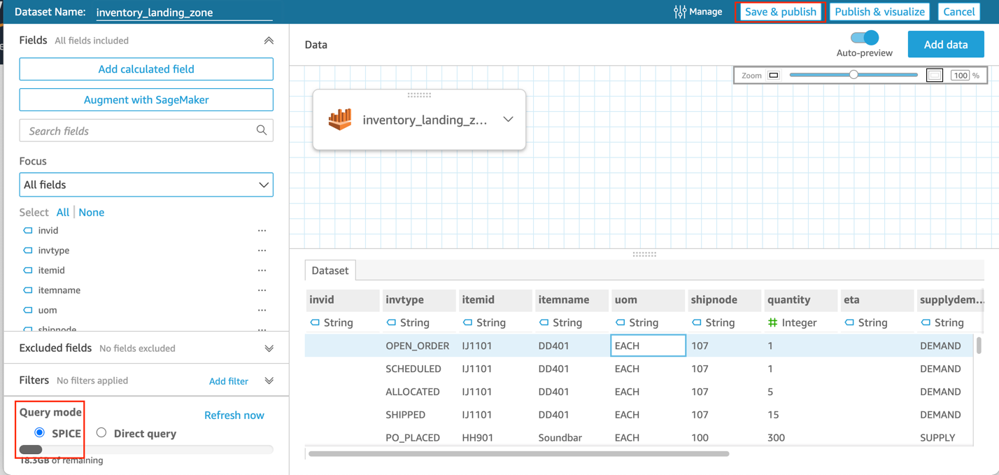\n\nBoth datasets should now be listed on the **Datasets** page.\n\n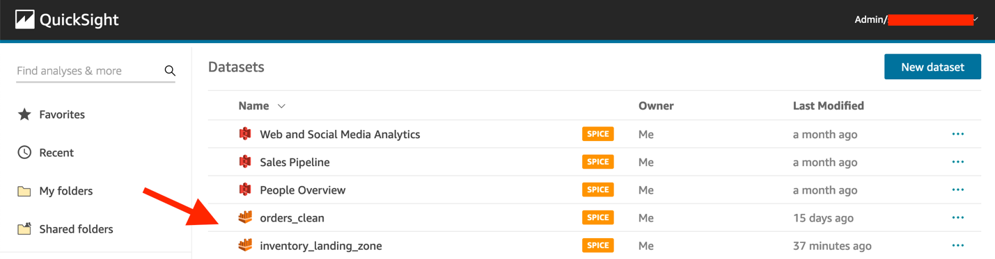\n\n22. Choose each dataset and choose **Refresh now**.\n\n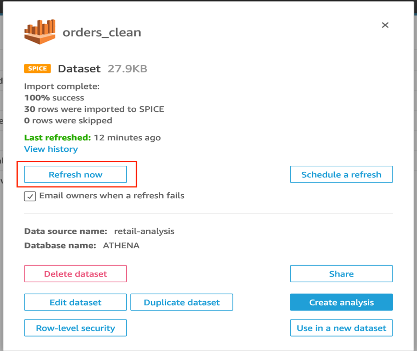\n\n23. Select **Full refresh** and choose **Refresh**.\n\n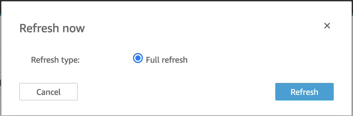\n\nTo set up a scheduled refresh, choose **Schedule a refresh** and provide your schedule details.\n\n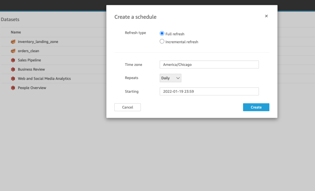\n\n##### **Create an analysis**\nTo create an analysis in QuickSight, complete the following steps:\n\n1. On the QuickSight console, choose **Analyses** in the navigation pane.\n2. Choose **New analysis**.\n\n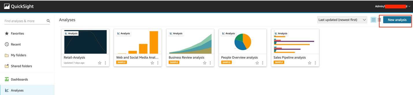\n\n3. Choose the ```orders_clean``` dataset.\n\n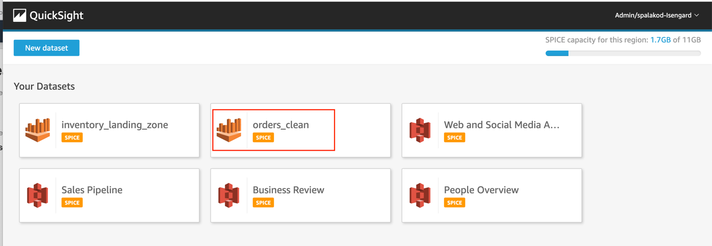\n\n4. Choose **Create analysis**.\n\n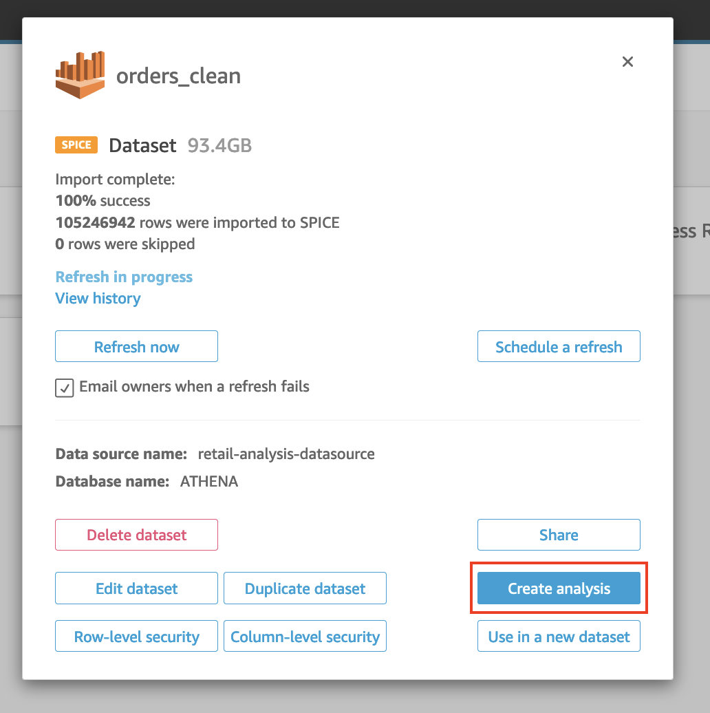\n\n5. To adjust the theme, choose **Themes** in the navigation pane, choose your preferred theme, and choose Apply.\n\n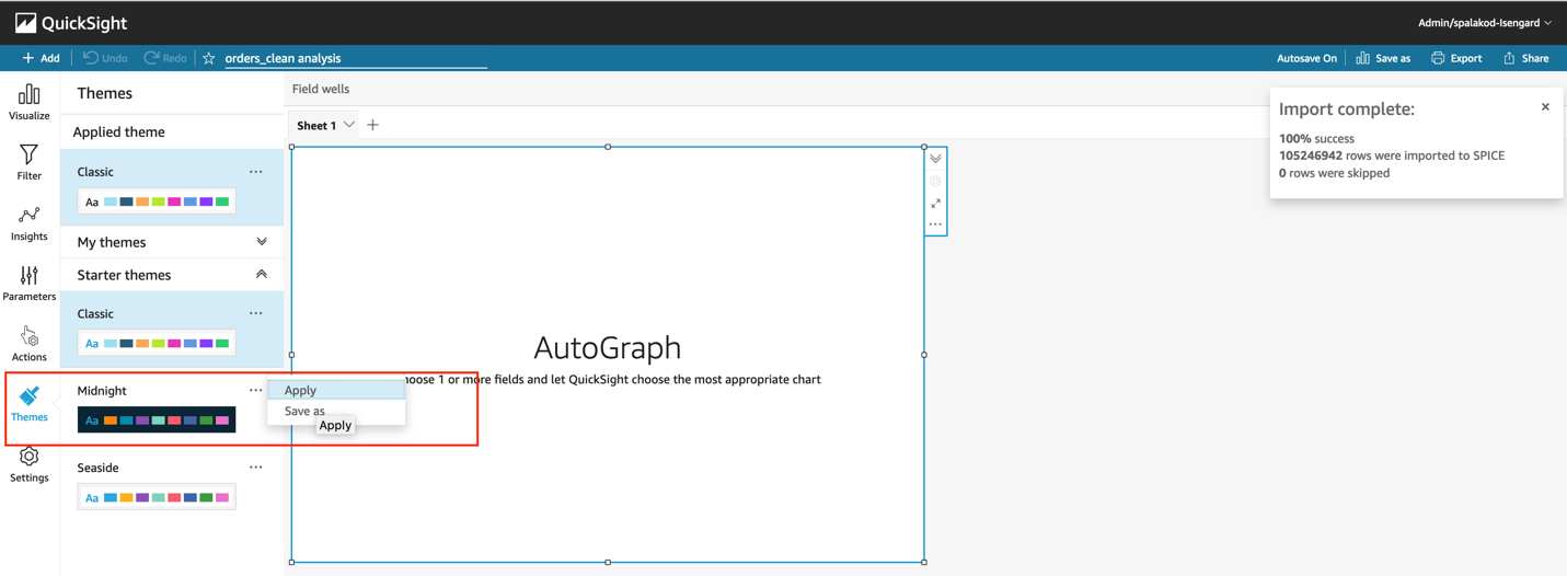\n\n6. Name the analysis ```retail-analysis```.\n\n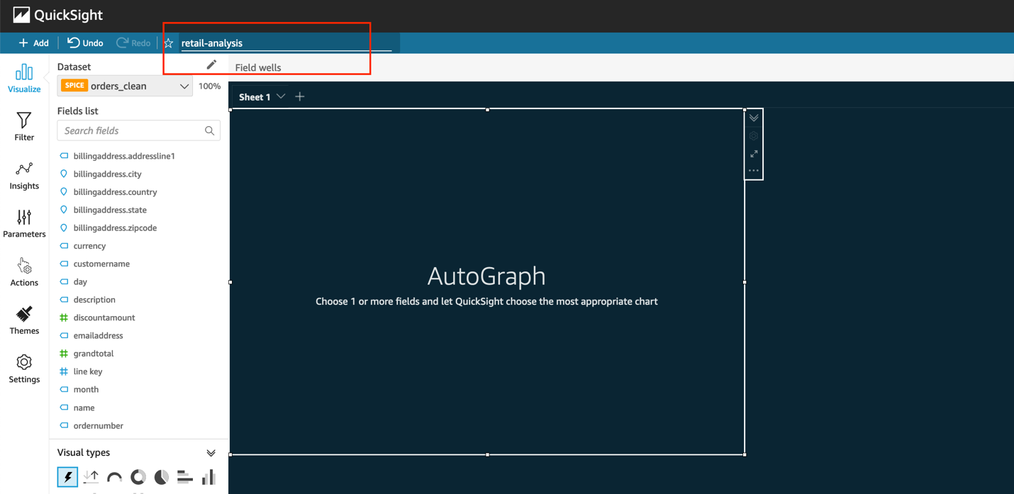\n\n##### **Add visualizations to the analysis**\n\nLet’s start creating visualizations. The first visualization shows orders created over time.\n\n1. Choose the empty graph on the dashboard and for Visual type¸ choose the line chart.\nFor more information about visual types, see [Visual types in Amazon QuickSight](https://docs.aws.amazon.com/quicksight/latest/user/working-with-visual-types.html).\n\n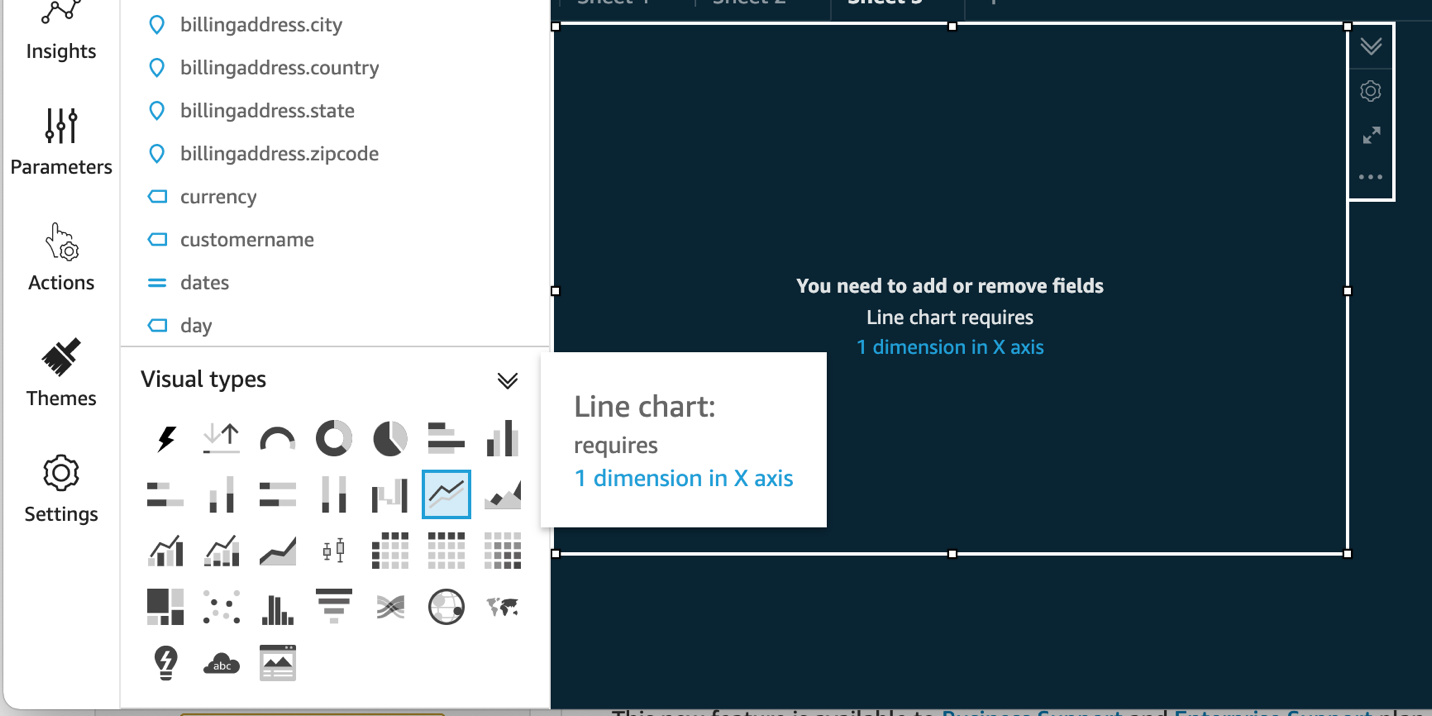\n\n2. Under **Field wells**, drag ```orderdatetime``` to X axis and ```ordernumber``` to Value.\n3. Set ```ordernumber``` to **Aggregate: Count distinct**.\n\n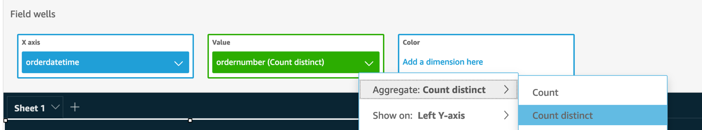\n\nNow we can filter these orders by ```Created``` status.\n4. Choose **Filter** in the navigation pane and choose **Create one**.\n5. Search for and choose **status**.\n\n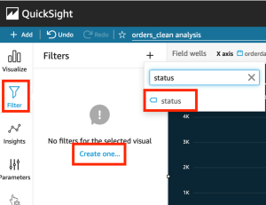\n\n6. Choose the **status** filter you just created.\n\n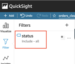\n\n7. Select **Created** from the filter list and choose **Apply**.\n\n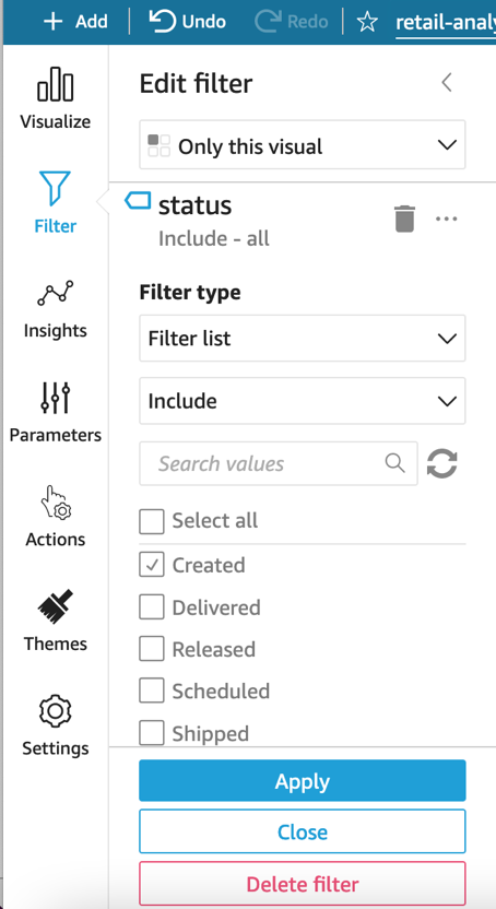\n\n8. Choose the graph (right-click) and choose **Add forecast**.\nThe forecasting ability is only available in the Enterprise Edition. QuickSight uses a built-in version of the Random Cut Forest (RCF) algorithm. For more information, refer to [Understanding the ML algorithm used by Amazon QuickSight](https://docs.aws.amazon.com/quicksight/latest/user/concept-of-ml-algorithms.html).\n\n\n\n9. Leave the settings as default and choose **Apply**.\n10. Rename the visualization to “Orders Created Over Time.”\n\nIf the forecast is applied successfully, the visualization shows the expected number of orders as well as upper and lower bounds.\n\n\n\nIf you get the following error message, allow for the data to accumulate for a few days before adding the forecast.\n\n\n\nLet’s create a visualization on orders by location.\n\n11. On the **Add** menu, choose **Add visual**.\n\n\n\n12. Choose the points on map visual type.\n\n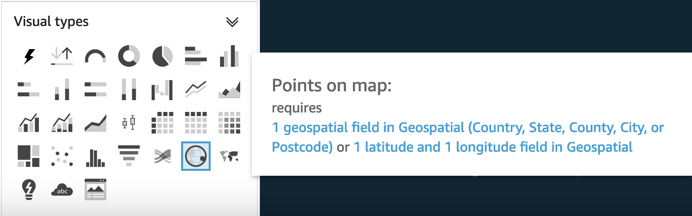\n\n13. Under **Field wells**, drag ```shippingaddress.zipcode``` to **Geospatial** and ```ordernumber to Size```.\n14. Change ```ordernumber``` to **Aggregate: Count distinct**.\n\n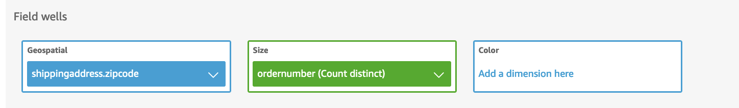\n\nYou should now see a map indicating the orders by location.\n\n15. Rename the visualization accordingly.\n\n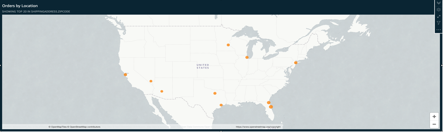\n\nNext, we create a drill-down visualization on the inventory count.\n\n16. Choose the pencil icon.\n\n\n\n17. Choose **Add dataset**.\n\n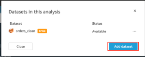\n\n18.Select the ```inventory_landing_zone``` dataset and choose **Select**.\n\n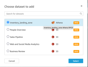\n\n19. Choose the ```inventory_landing_zone``` dataset.\n\n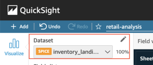\n\n20. Add the vertical bar chart visual type.\n\n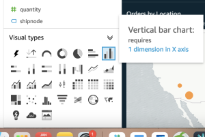\n\n21. Under **Field wells**, drag ```itemname```, ```shipnode```, and ```invtype``` to **X axis**, and quantity to **Value**.\n22. Make sure that quantity is set to **Sum**.\n\n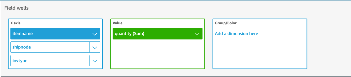\n\nThe following screenshot shows an example visualization of order inventory.\n\n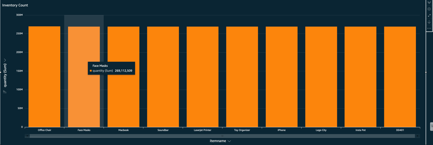\n\n23. To determine how many face masks were shipped out from each ship node, choose **Face Masks** (right-click) and choose **Drill down to shipnode**.\n\n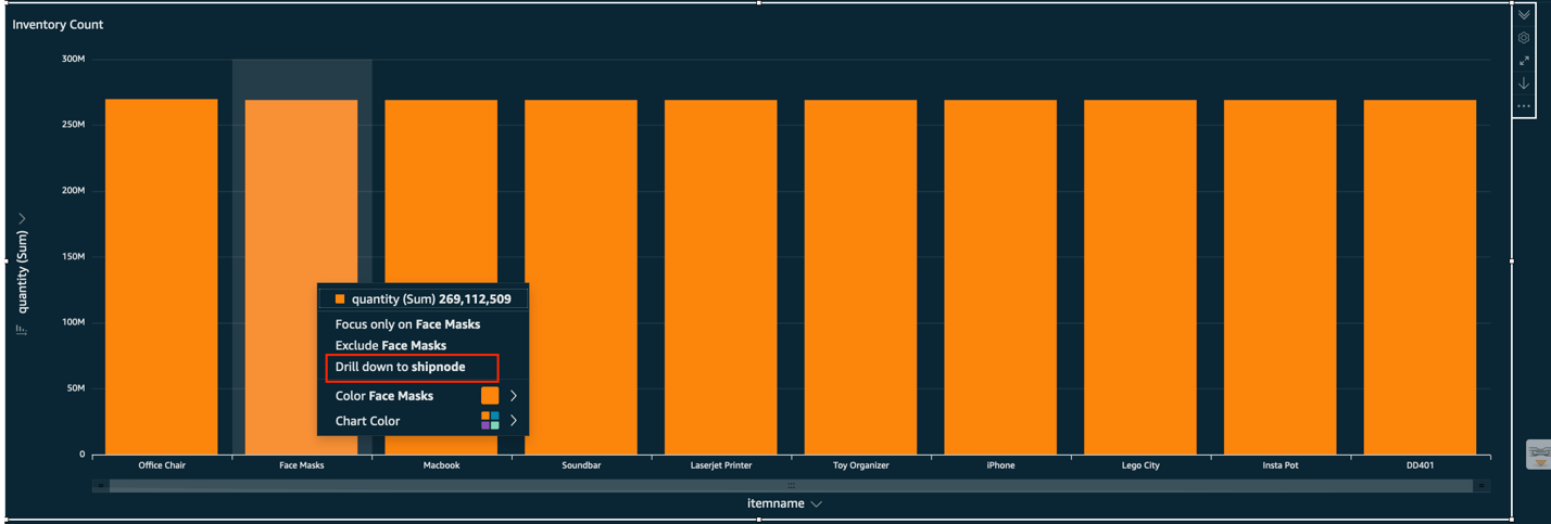\n\n24. You can drill down even further to ```invtype``` to see how many face masks in a specific ship node are in which status.\n\n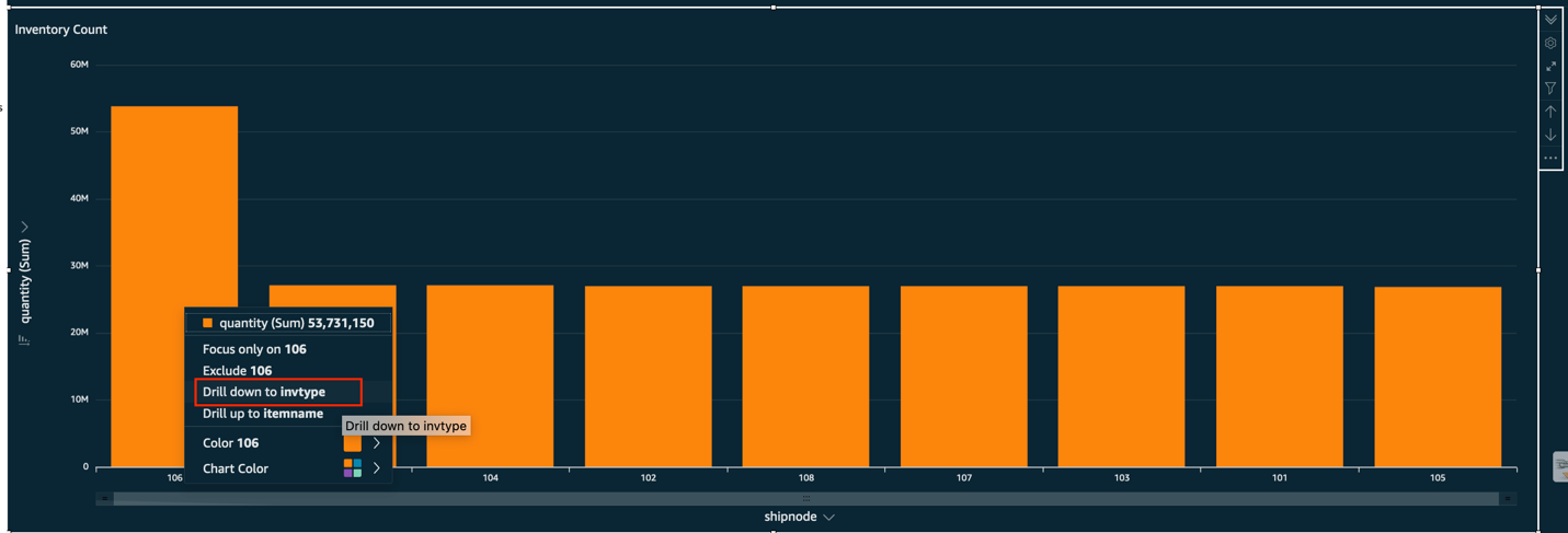\n\nThe following screenshot shows this drilled-down inventory count.\n\n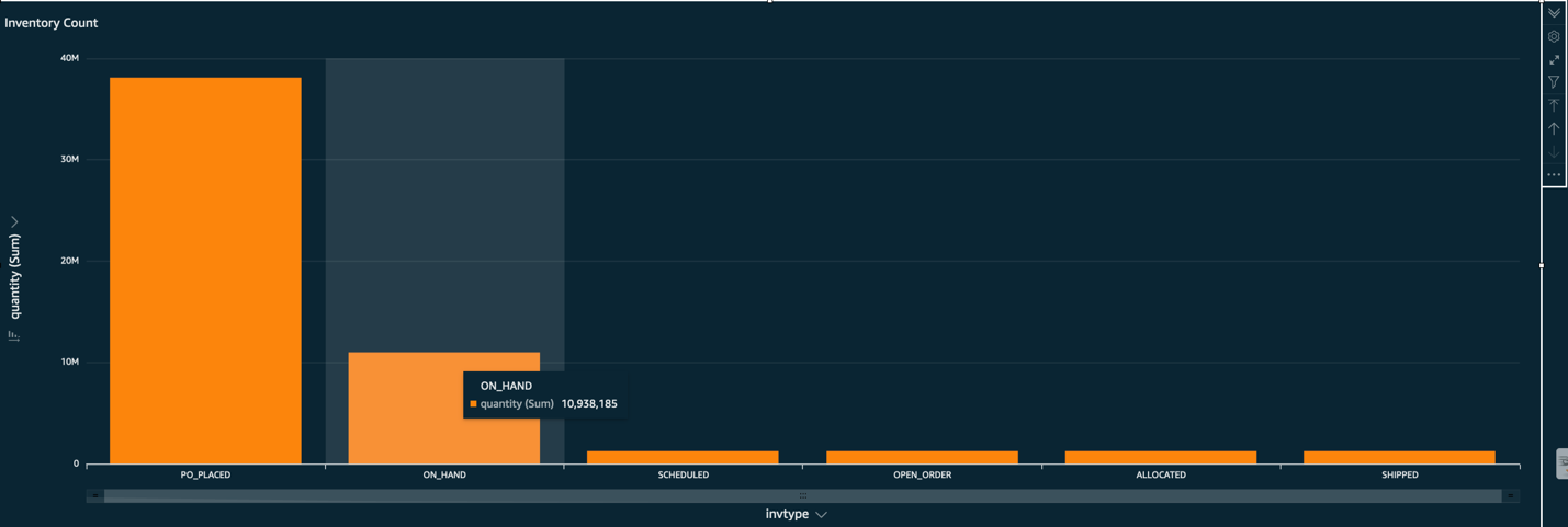\n\nAs a next step, you can create a QuickSight dashboard from the analysis you created. For instructions, refer to [Tutorial: Create an Amazon QuickSight dashboard](https://docs.aws.amazon.com/quicksight/latest/user/example-create-a-dashboard.html).\n\n#### **Clean up**\nTo avoid any ongoing charges, on the AWS CloudFormation console, select the stack you created and choose **Delete**. This deletes all the created resources. On the stack’s **Events** tab, you can track the progress of the deletion, and wait for the stack status to change to ```DELETE_COMPLETE```.\n\nThe Amazon EventBridge rules generate orders and inventory data every 15 minutes, to avoid generating huge amount of data, please ensure to delete the stack after testing the blog.\n\nIf the deletion of any resources fails, ensure that you delete them manually. For deleting Amazon QuickSight datasets, you can follow [these instructions](https://docs.aws.amazon.com/quicksight/latest/user/delete-a-data-set.html). You can delete the QuickSight Analysis using [these steps](https://docs.aws.amazon.com/quicksight/latest/user/deleting-an-analysis.html). For deleting the QuickSight subscription and closing the account, you can follow [these instructions](https://docs.aws.amazon.com/quicksight/latest/user/closing-account.html).\n\n#### **Conclusion**\nIn this post, we showed you how to use AWS analytics and storage services to build a serverless operational data lake. Kinesis Data Streams lets you ingest large volumes of data, and DataBrew lets you cleanse and transform the data visually. We also showed you how to analyze and visualize the order and inventory data using AWS Glue, Athena, and QuickSight. For more information and resources for data lakes on AWS, visit [Analytics on AWS](https://aws.amazon.com/big-data/datalakes-and-analytics/).\n\n##### **About the Authors**\n\n\n\n**Gandhi Raketla** is a Senior Solutions Architect for AWS. He works with AWS customers and partners on cloud adoption, as well as architecting solutions that help customers foster agility and innovation. He specializes in the AWS data analytics domain.\n\n\n\n**Sindhura Palakodety** is a Solutions Architect at AWS. She is passionate about helping customers build enterprise-scale Well-Architected solutions on the AWS Cloud and specializes in the containers and data analytics domains.\n","render":"<p>Do you want to reduce stockouts at stores? Do you want to improve order delivery timelines? Do you want to provide your customers with accurate product availability, down to the millisecond? A retail operational data lake can help you transform the customer experience by providing deeper insights into a variety of operational aspects of your supply chain.</p>\n<p>In this post, we demonstrate how to create a serverless operational data lake using AWS services, including <a href=\"https://aws.amazon.com/glue\" target=\"_blank\">AWS Glue</a>, Amazon Kinesis Data Streams, <a href=\"https://aws.amazon.com/dynamodb/\" target=\"_blank\">Amazon DynamoDB</a>, <a href=\"https://aws.amazon.com/athena/\" target=\"_blank\">Amazon Athena</a>, and <a href=\"https://aws.amazon.com/quicksight\" target=\"_blank\">Amazon QuickSight</a>.</p>\n<p>Retail operations is a critical functional area that gives retailers a competitive edge. An efficient retail operation can optimize the supply chain for a better customer experience and cost reduction. An optimized retail operation can reduce frequent stockouts and delayed shipments, and provide accurate inventory and order details. Today, a retailer’s channels aren’t just store and web—they include mobile apps, chatbots, connected devices, and social media channels. The data is both structured and unstructured. This coupled with multiple fulfillment options like buy online and pick up at store, ship from store, or ship from distribution centers, which increases the complexity of retail operations.</p>\n<p>Most retailers use a centralized order management system (OMS) for managing orders, inventory, shipments, payments, and other operational aspects. These legacy OMSs are unable to scale in response to the rapid changes in retail business models. The enterprise applications that are key for efficient and smooth retail operations rely on a central OMS. Applications for ecommerce, warehouse management, call centers, and mobile all require an OMS to get order status, inventory positions of different items, shipment status, and more. Another challenge with legacy OMSs is they’re not designed to handle unstructured data like weather data and IoT data that could impact inventory and order fulfillment. A legacy OMS that can’t scale prohibits you from implementing new business models that could transform your customer experience.</p>\n<p>A data lake is a centralized repository that allows you to store all your structured and unstructured data at any scale. An operational data lake addresses this challenge by providing easy access to structured and unstructured operational data in real time from various enterprise systems. You can store your data as is, without having to first structure the data, and run different types of analytics—from dashboards and visualizations to big data processing, real-time analytics, and machine learning (ML)—to guide better decisions. This can ease the burden on OMSs that can instead focus on order orchestration and management.</p>\n<h4><a id=\"Solution_overview_10\"></a><strong>Solution overview</strong></h4>\n<p>In this post, we create an end-to-end pipeline to ingest, store, process, analyze, and visualize operational data like orders, inventory, and shipment updates. We use the following AWS services as key components:</p>\n<ul>\n<li>Kinesis Data Streams to ingest all operational data in real time from various systems</li>\n<li>DynamoDB, <a href=\"https://aws.amazon.com/rds/aurora/\" target=\"_blank\">Amazon Aurora</a>, and <a href=\"http://aws.amazon.com/s3\" target=\"_blank\">Amazon Simple Storage Service</a> (Amazon S3) to store the data</li>\n<li><a href=\"https://aws.amazon.com/glue/features/databrew/\" target=\"_blank\">AWS Glue DataBrew</a> to clean and transform the data</li>\n<li>AWS Glue crawlers to catalog the data</li>\n<li>Athena to query the processed data</li>\n<li>A QuickSight dashboard that provides insights into various operational metrics</li>\n</ul>\n<p>The following diagram illustrates the solution architecture.</p>\n<p><img src=\"https://dev-media.amazoncloud.cn/15adb6058de34f98b3135df3693aaa2d_image.png\" alt=\"image.png\" /></p>\n<p>The data pipeline consists of stages to ingest, store, process, analyze, and finally visualize the data, which we discuss in more detail in the following sections.</p>\n<h4><a id=\"Data_ingestion_26\"></a><strong>Data ingestion</strong></h4>\n<p>Orders and inventory data is ingested in real time from multiple sources like web applications, mobile apps, and connected devices into Kinesis Data Streams. Kinesis Data Streams is a massively scalable and durable real-time data streaming service. Kinesis Data Streams can continuously capture gigabytes of data per second from hundreds of thousands of sources, such as web applications, database events, inventory transactions, and payment transactions. Frontend systems like ecommerce applications and mobile apps ingest the order data as soon as items are added to a cart or an order is created. The OMS ingests orders when the order status changes. OMSs, stores, and third-party suppliers ingest inventory updates into the data stream.</p>\n<p>To simulate orders, an <a href=\"http://aws.amazon.com/lambda\" target=\"_blank\">AWS Lambda</a> function is triggered by a scheduled <a href=\"http://aws.amazon.com/cloudwatch\" target=\"_blank\">Amazon CloudWatch</a> event every minute to ingest orders to a data stream. This function simulates the typical order management system lifecycle (order created, scheduled, released, shipped, and delivered). Similarly, a second Lambda function is triggered by a CloudWatch event to generate inventory updates. This function simulates different inventory updates such as purchase orders created from systems like the OMS or third-party suppliers. In a production environment, this data would come from frontend applications and a centralized order management system.</p>\n<h4><a id=\"Data_storage_31\"></a><strong>Data storage</strong></h4>\n<p>There are two types of data: hot and cold data. Hot data is consumed by frontend applications like web applications, mobile apps, and connected devices. The following are some example use cases for hot data:</p>\n<ul>\n<li>When a customer is browsing products, the real-time availability of the item must be displayed</li>\n<li>Customers interacting with Alexa to know the status of the order</li>\n<li>A call center agent interacting with a customer needs to know the status of the customer order or its shipment details</li>\n</ul>\n<p>The systems, APIs, and devices that consume this data need the data within seconds or milliseconds of the transactions.</p>\n<p>Cold data is used for long-term analytics like orders over a period of time, orders by channel, top 10 items by number of orders, or planned vs. available inventory by item, warehouse, or store.</p>\n<p>For this solution, we store orders hot data in DynamoDB. DynamoDB is a fully managed NoSQL database that delivers single-digit millisecond performance at any scale. A Lambda function processes records in the Kinesis data stream and stores it in a DynamoDB table.</p>\n<p>Inventory hot data is stored in an <a href=\"https://aws.amazon.com/rds/aurora/mysql-features/\" target=\"_blank\">Amazon Aurora MySQL-Compatible Edition</a> database. Inventory is transactional data that requires high consistency so that customers aren’t over-promised or under-promised when they place orders. Aurora MySQL is fully managed database that is up to five times faster than standard MySQL databases and three times faster than standard PostgreSQL databases. It provides the security, availability, and reliability of commercial databases at a tenth of the cost.</p>\n<p>Amazon S3 is object storage built to store and retrieve any amount of data from anywhere. It’s a simple storage service that offers industry-leading durability, availability, performance, security, and virtually unlimited scalability at very low cost. Order and inventory cold data is stored in Amazon S3.</p>\n<p><a href=\"https://aws.amazon.com/kinesis/data-firehose/\" target=\"_blank\">Amazon Kinesis Data</a> Firehose reads the data from the Kinesis data stream and stores it in Amazon S3. Kinesis Data Firehose is the easiest way to load streaming data into data stores and analytics tools. It can capture, transform, and load streaming data into Amazon S3, <a href=\"http://aws.amazon.com/redshift\" target=\"_blank\">Amazon Redshift</a>, <a href=\"https://aws.amazon.com/opensearch-service/\" target=\"_blank\">Amazon OpenSearch Service</a>, and Splunk, enabling near-real-time analytics.</p>\n<p><strong>Data processing</strong><br />\nThe data processing stage involves cleaning, preparing, and transforming the data to help downstream analytics applications easily query the data. Each frontend system might have a different data format. In the data processing stage, data is cleaned and converted into a common canonical form.</p>\n<p>For this solution, we use DataBrew to clean and convert orders into a common canonical form. DataBrew is a visual data preparation tool that makes it easy for data analysts and data scientists to prepare data with an interactive, point-and-click visual interface without writing code. DataBrew provides over 250 built-in transformations to combine, pivot, and transpose the data without writing code. The cleaning and transformation steps in DataBrew are called recipes. A scheduled DataBrew job applies the recipes to the data in an S3 bucket and stores the output in a different bucket.</p>\n<p>AWS Glue crawlers can access data stores, extract metadata, and create table definitions in the AWS Glue Data Catalog. You can schedule a crawler to crawl the transformed data and create or update the Data Catalog. The AWS Glue Data Catalog is your persistent metadata store. It’s a managed service that lets you store, annotate, and share metadata in the AWS Cloud in the same way you would in an Apache Hive metastore. We use crawlers to populate the Data Catalog with tables.</p>\n<p><strong>Data analysis</strong><br />\nWe can query orders and inventory data from S3 buckets using Athena. Athena is an interactive query service that makes it easy to analyze data in Amazon S3 using standard SQL. Athena is serverless, so there is no infrastructure to manage, and you pay only for the queries that you run. Views are created in Athena that can be consumed by business intelligence (BI) services like QuickSight.</p>\n<p><strong>Data visualization</strong><br />\nWe generate dashboards using QuickSight. QuickSight is a scalable, serverless, embeddable BI service powered by ML and built for the cloud. QuickSight lets you easily create and publish interactive BI dashboards that include ML-powered insights.</p>\n<p>QuickSight also has features to forecast orders, detect anomalies in the order, and provide ML-powered insights. We can create analyses such as orders over a period of time, orders split by channel, top 10 locations for orders, or order fulfillment timelines (the time it took from order creation to order delivery).</p>\n<h4><a id=\"Walkthrough_overview_65\"></a><strong>Walkthrough overview</strong></h4>\n<p>To implement this solution, you complete the following high-level steps:</p>\n<ol>\n<li>Create solution resources using <a href=\"http://aws.amazon.com/cloudformation\" target=\"_blank\">AWS CloudFormation</a>.</li>\n<li>Connect to the inventory database.</li>\n<li>Load the inventory database with tables.</li>\n<li>Create a <a href=\"https://docs.aws.amazon.com/vpc/latest/privatelink/vpc-endpoints.html\" target=\"_blank\">VPC endpoint</a> using <a href=\"http://aws.amazon.com/vpc\" target=\"_blank\">Amazon Virtual Private Cloud</a> (Amazon VPC).</li>\n<li>Create <a href=\"https://docs.aws.amazon.com/vpc/latest/privatelink/vpce-gateway.html\" target=\"_blank\">gateway endpoints</a> for Amazon S3 on the default VPC.</li>\n<li>Enable CloudWatch rules via <a href=\"https://aws.amazon.com/eventbridge/\" target=\"_blank\">Amazon EventBridge</a> to ingest the data.</li>\n<li>Transform the data using AWS Glue.</li>\n<li>Visualize the data with QuickSight.</li>\n</ol>\n<h4><a id=\"Prerequisites_77\"></a><strong>Prerequisites</strong></h4>\n<p>Complete the following prerequisite steps:</p>\n<ol>\n<li>Create AWS account if you don’t have done already.</li>\n<li><a href=\"https://docs.aws.amazon.com/quicksight/latest/user/signing-up.html\" target=\"_blank\">Sign up for QuickSight</a> if you’ve never used QuickSight in this account before. To use the forecast ability in QuickSight, sign up for the Enterprise Edition.</li>\n</ol>\n<h4><a id=\"Create_resources_with_AWS_CloudFormation_83\"></a><strong>Create resources with AWS CloudFormation</strong></h4>\n<p>To launch the provided CloudFormation template, complete the following steps:</p>\n<ol>\n<li>Choose <strong>Launch Stack</strong>:<br />\n<a href=\"https://console.aws.amazon.com/cloudformation/home?region=us-east-1#/stacks/create/template?stackName=operational-data-lake&amp;templateURL=https://aws-blogs-artifacts-public.s3.amazonaws.com/artifacts/BDB-1266/Datalake_Blog_CF.yaml\" target=\"_blank\"><img src=\"https://dev-media.amazoncloud.cn/7623c30018444331b7e03ce2a6d68ee1_image.png\" alt=\"image.png\" /></a></li>\n<li>Choose <strong>Next</strong>.</li>\n<li>For <strong>Stack name</strong>, enter a name.</li>\n<li>Provide the following parameters:\n<ul>\n<li>The name of the S3 bucket that holds all the data for the data lake.The</li>\n<li>name of the database that holds the inventory tables.</li>\n<li>The database user name.</li>\n<li>The database password.</li>\n</ul>\n</li>\n<li>Enter any tags you want to assign to the stack and choose <strong>Next</strong>.</li>\n<li>Select the acknowledgement check boxes and choose <strong>Create stack</strong>.</li>\n</ol>\n<p>The stack takes 5–10 minutes to complete.</p>\n<p>On the AWS CloudFormation console, you can navigate to the stack’s <strong>Outputs</strong> tab to review the resources you created.</p>\n<p><img src=\"https://dev-media.amazoncloud.cn/3b3b1c708e4c4fd591717a585627a356_image.png\" alt=\"image.png\" /></p>\n<p>If you open the S3 bucket you created, you can observe its folder structure. The stack creates sample order data for the last 7 days.</p>\n<p><img src=\"https://dev-media.amazoncloud.cn/7417ed4f44134ef5af4fd331e5b6f454_image.png\" alt=\"image.png\" /></p>\n<h4><a id=\"Connect_to_the_inventory_database_108\"></a><strong>Connect to the inventory database</strong></h4>\n<p>To connect to your database in the query editor, complete the following steps:</p>\n<ol>\n<li>On the Amazon RDS console, choose the Region you deployed the stack in.</li>\n</ol>\n<p><img src=\"https://dev-media.amazoncloud.cn/8e69b92846664116bce983d011f4f47a_image.png\" alt=\"image.png\" /></p>\n<ol start=\"2\">\n<li>In the navigation pane, choose <strong>Query Editor</strong>.</li>\n</ol>\n<p><img src=\"https://dev-media.amazoncloud.cn/ad947017ac4a4ddb894fa6713a316110_image.png\" alt=\"image.png\" /></p>\n<p>If you haven’t connected to this database before, the <strong>Connect to database</strong> page opens.</p>\n<ol start=\"3\">\n<li>For <strong>Database instance</strong> or cluster, choose your database.</li>\n<li>For <strong>Database username</strong>, choose <strong>Connect with a Secrets Manager ARN</strong>.<br />\nThe database user name and password provided during stack creation are stored in AWS Secrets Manager. Alternatively, you can choose Add new database credentials and enter the database user name and password you provided when creating the stack.</li>\n<li>For <strong>Secrets Manager ARN</strong>, enter the value for the key <code>InventorySecretManager</code> from the CloudFormation stack outputs.</li>\n<li>Optionally, enter the name of your database.</li>\n<li>Choose <strong>Connect to database</strong>.</li>\n</ol>\n<p><img src=\"https://dev-media.amazoncloud.cn/7ef175c9f1444465b2d720356466fcf4_image.png\" alt=\"image.png\" /></p>\n<h4><a id=\"Load_the_inventory_database_with_tables_131\"></a><strong>Load the inventory database with tables</strong></h4>\n<p>Enter the following DDL statement in the query editor and choose <strong>Run</strong>:</p>\n<pre><code class=\"lang-\">CREATE TABLE INVENTORY (\n ItemID varchar(25) NOT NULL,\n ShipNode varchar(25) NOT NULL,\n SupplyType varchar(25) NOT NULL,\n SupplyDemandType varchar(25) NOT NULL,\n ItemName varchar(25),\n UOM varchar(10),\n Quantity int(11) NOT NULL,\n ETA varchar(25)\t ,\n UpdatedDate DATE,\n PRIMARY KEY (ItemID,ShipNode,SupplyType)\n);\n</code></pre>\n<p><img src=\"https://dev-media.amazoncloud.cn/f6a19a2a6cd64f998d81237bd4dfcfc7_image.png\" alt=\"image.png\" /></p>\n<h4><a id=\"Create_a_VPC_endpoint_151\"></a><strong>Create a VPC endpoint</strong></h4>\n<p>To create your VPC endpoint, complete the following steps:</p>\n<ol>\n<li>On the Amazon VPC console, choose <strong>VPC Dashboard</strong>.</li>\n<li>Choose <strong>Endpoints</strong> in the navigation pane.</li>\n<li>Choose <strong>Create Endpoint</strong>.</li>\n</ol>\n<p><img src=\"https://dev-media.amazoncloud.cn/80b8284d27b44c818318b5b585f56b28_image.png\" alt=\"image.png\" /></p>\n<ol start=\"4\">\n<li>For <strong>Service category</strong>, select <strong>AWS services</strong>.</li>\n<li>For <strong>Service name</strong>, search for <code>rds</code> and choose the service name ending with <code>rds-data</code>.</li>\n<li>For <strong>VPC</strong>, choose <strong>the default VPC</strong>.</li>\n</ol>\n<p><img src=\"https://dev-media.amazoncloud.cn/8a93677d9b004cb68ea44950a990ba73_image.png\" alt=\"image.png\" /></p>\n<ol start=\"7\">\n<li>Leave the remaining settings at their default and choose <strong>Create endpoint</strong>.</li>\n</ol>\n<h4><a id=\"Create_a_gateway_endpoint_for_Amazon_S3_168\"></a><strong>Create a gateway endpoint for Amazon S3</strong></h4>\n<p>To create your gateway endpoint, complete the following steps:</p>\n<ol>\n<li>On the Amazon VPC console, choose <strong>VPC Dashboard</strong>.</li>\n<li>Choose <strong>Endpoints</strong> in the navigation pane.</li>\n<li>Choose <strong>Create Endpoint</strong>.</li>\n<li>For <strong>Service category</strong>, select <strong>AWS services</strong>.\n<ol>\n<li>For <strong>Service name</strong>, search for <code>S3</code> and choose the service name with type <strong>Gateway</strong>.</li>\n</ol>\n</li>\n<li>For <strong>VPC</strong>, choose the default VPC.</li>\n<li>For <strong>Configure route tables</strong>, select the default route table.</li>\n</ol>\n<p><img src=\"https://dev-media.amazoncloud.cn/ebc7481c62864d658e20627a5a1e9f56_image.png\" alt=\"image.png\" /></p>\n<ol start=\"8\">\n<li>Leave the remaining settings at their default and choose <strong>Create endpoint</strong>.</li>\n</ol>\n<p>Wait for both the gateway endpoint and VPC endpoint status to change to <code>Available</code>.</p>\n<p><img src=\"https://dev-media.amazoncloud.cn/50c3202a656c42e193a9bb04d5d862a0_image.png\" alt=\"image.png\" /></p>\n<h4><a id=\"Enable_CloudWatch_rules_to_ingest_the_data_187\"></a><strong>Enable CloudWatch rules to ingest the data</strong></h4>\n<p>We created two CloudWatch rules via the CloudFormation template to ingest the order and inventory data to Kinesis Data Streams. To enable the rules via EventBridge, complete the following steps:</p>\n<ol>\n<li>On the CloudWatch console, under <strong>Events</strong> in the navigation pane, choose <strong>Rules</strong>.</li>\n<li>Make sure you’re in the Region where you created the stack.</li>\n<li>Choose <strong>Go to Amazon EventBridge</strong>.</li>\n</ol>\n<p><img src=\"https://dev-media.amazoncloud.cn/b61f69708a4441e1ac1de5be549b6ce0_image.png\" alt=\"image.png\" /></p>\n<ol start=\"4\">\n<li>Select the rule <code>Ingest-Inventory-Update-Schedule-Rule</code> and choose <strong>Enable</strong>.</li>\n<li>Select the rule <code>Ingest-Order-Schedule-Rule</code> and choose <strong>Enable</strong>.</li>\n</ol>\n<p><img src=\"https://dev-media.amazoncloud.cn/5737a46bdb884e06b1636f30ad4ee0a3_image.png\" alt=\"image.png\" /></p>\n<p>After 5–10 minutes, the Lambda functions start ingesting orders and inventory updates to their respective streams. You can check the S3 buckets <code>orders-landing-zone</code> and <code>inventory-landing-zone</code> to confirm that the data is being populated.</p>\n<h4><a id=\"Perform_data_transformation_203\"></a><strong>Perform data transformation</strong></h4>\n<p>Our CloudFormation stack included a DataBrew project, a DataBrew job that runs every 5 minutes, and two AWS Glue crawlers. To perform data transformation using our AWS Glue resources, complete the following steps:</p>\n<ol>\n<li>On the DataBrew console, choose <strong>Projects</strong> in the navigation pane.</li>\n<li>Choose the project <code>OrderDataTransform</code>.</li>\n</ol>\n<p><img src=\"https://dev-media.amazoncloud.cn/8d48fef7c2df4877981907492144bea3_image.png\" alt=\"image.png\" /></p>\n<p>You can review the project and its recipe on this page.</p>\n<p><img src=\"https://dev-media.amazoncloud.cn/6f1a1aecb44043ff8132e1f2fe641530_image.png\" alt=\"image.png\" /></p>\n<ol start=\"3\">\n<li>In the navigation pane, choose <strong>Jobs</strong>.</li>\n<li>Review the job status to confirm it’s complete.</li>\n</ol>\n<p><img src=\"https://dev-media.amazoncloud.cn/edb19d0d4d2d411d839ef5632da69de3_image.png\" alt=\"image.png\" /></p>\n<ol start=\"5\">\n<li>On the AWS Glue console, choose <strong>Crawlers</strong> in the navigation pane.<br />\nThe crawlers crawl the transformed data and update the Data Catalog.</li>\n<li>Review the status of the two crawlers, which run every 15 minutes.</li>\n</ol>\n<p><img src=\"https://dev-media.amazoncloud.cn/b39fb02cde884736a5ff25ba5fe12712_image.png\" alt=\"image.png\" /></p>\n<ol start=\"7\">\n<li>Choose <strong>Tables</strong> in the navigation pane to view the two tables the crawlers created.<br />\nIf you don’t see these tables, you can run the crawlers manually to create them.</li>\n</ol>\n<p><img src=\"https://dev-media.amazoncloud.cn/7f2d427448ee49039633f7402c7dca1c_image.png\" alt=\"image.png\" /></p>\n<p>You can query the data in the tables with Athena.<br />\n8. On the Athena console, choose <strong>Query editor</strong>.<br />\nIf you haven’t created a query result location, you’re prompted to do that first.<br />\n9. Choose <strong>View settings</strong> or choose the <strong>Settings tab</strong>.</p>\n<p><img src=\"https://dev-media.amazoncloud.cn/13b9c69d1787449ebeaa8fdfe62d6b0e_image.png\" alt=\"image.png\" /></p>\n<ol start=\"10\">\n<li>Choose <strong>Manage</strong>.</li>\n</ol>\n<p><img src=\"https://dev-media.amazoncloud.cn/1e444cc50cb84387826850f9bfa3513c_image.png\" alt=\"image.png\" /></p>\n<ol start=\"11\">\n<li>Select the S3 bucket to store the results and choose <strong>Choose</strong>.</li>\n</ol>\n<p><img src=\"https://dev-media.amazoncloud.cn/3b285bc2705f4f64a58422628881dfb8_image.png\" alt=\"image.png\" /></p>\n<ol start=\"12\">\n<li>Choose <strong>Query editor</strong> in the navigation pane.</li>\n</ol>\n<p><img src=\"https://dev-media.amazoncloud.cn/809c1b0e65e643d3b84d14fee200fbd3_image.png\" alt=\"image.png\" /></p>\n<p>13.Choose either table (right-click) and choose <strong>Preview Table</strong> to view the table contents.</p>\n<p><img src=\"https://dev-media.amazoncloud.cn/3730d858c53f4fbfaec3a28823ac4c98_image.png\" alt=\"image.png\" /></p>\n<h4><a id=\"Visualize_the_data_254\"></a><strong>Visualize the data</strong></h4>\n<p>If you have never used QuickSight in this account before, complete the prerequisite step to sign up for QuickSight. To use the ML capabilities of QuickSight (such as <a href=\"https://docs.aws.amazon.com/quicksight/latest/user/forecasts-and-whatifs.html\" target=\"_blank\">forecasting</a>) sign up for the Enterprise Edition using the steps in this <a href=\"https://docs.aws.amazon.com/quicksight/latest/user/signing-up.html\" target=\"_blank\">documentation</a>.</p>\n<p>While signing up for QuickSight, make sure to use the <strong>same region</strong> where you created the CloudFormation stack.</p>\n<h5><a id=\"Grant_QuickSight_permissions_259\"></a><strong>Grant QuickSight permissions</strong></h5>\n<p>To visualize your data, you must first grant relevant permissions to QuickSight to access your data.</p>\n<ol>\n<li>On the QuickSight console, on the Admin drop-down menu, choose <strong>Manage QuickSight</strong>.</li>\n</ol>\n<p><img src=\"https://dev-media.amazoncloud.cn/2aab31c11c8249eeba5337c48f3b61e9_image.png\" alt=\"image.png\" /></p>\n<ol start=\"2\">\n<li>In the navigation pane, choose <strong>Security &amp; permissions</strong>.</li>\n<li>Under <strong>QuickSight access to AWS services</strong>, choose <strong>Manage</strong>.</li>\n</ol>\n<p><img src=\"https://dev-media.amazoncloud.cn/6615c458c5b940a8897c59ead7b8cd49_image.png\" alt=\"image.png\" /></p>\n<ol start=\"4\">\n<li>Select <strong>Amazon Athena</strong>.</li>\n<li>Select <strong>Amazon S3</strong> to edit QuickSight access to your S3 buckets.</li>\n<li>Select the bucket you specified during stack creation (for this post, <code>operational-datalake</code>).</li>\n<li>Choose <strong>Finish</strong>.</li>\n</ol>\n<p><img src=\"https://dev-media.amazoncloud.cn/3519754a55fa4d4e94ea6d37f134e926_image.png\" alt=\"image.png\" /></p>\n<ol start=\"8\">\n<li>Choose <strong>Save</strong>.</li>\n</ol>\n<h5><a id=\"Prepare_the_datasets_280\"></a><strong>Prepare the datasets</strong></h5>\n<p>To prepare your datasets, complete the following steps:</p>\n<ol>\n<li>On the QuickSight console, choose <strong>Datasets</strong> in the navigation pane.</li>\n<li>Choose <strong>New dataset</strong>.</li>\n</ol>\n<p><img src=\"https://dev-media.amazoncloud.cn/defe7368d7a04850b1f728fd2998adc0_image.png\" alt=\"image.png\" /></p>\n<p>3.Choose <strong>Athena</strong>.</p>\n<p><img src=\"https://dev-media.amazoncloud.cn/9b01ecbf3d114980896a8382f01c8e22_image.png\" alt=\"image.png\" /></p>\n<ol start=\"4\">\n<li>For <strong>Data source name</strong>, enter <code>retail-analysis</code>.</li>\n<li>Choose <strong>Validate connection</strong>.</li>\n<li>After your connection is validated, choose <strong>Create data source</strong>.</li>\n</ol>\n<p>For Data source name, enter retail-analysis.<br />\nChoose Validate connection.<br />\nAfter your connection is validated, choose Create data source.</p>\n<ol start=\"7\">\n<li>For <strong>Database</strong>, choose orderdatalake.</li>\n<li>For <strong>Tables</strong>, select <code>orders_clean</code>.</li>\n<li>Choose <strong>Edit/Preview data</strong>.</li>\n</ol>\n<p><img src=\"https://dev-media.amazoncloud.cn/c661a3d8651e4af8a56aa1fc98205233_image.png\" alt=\"image.png\" /></p>\n<ol start=\"10\">\n<li>For <strong>Query mode</strong>, select <strong>SPICE</strong>.<br />\n<a href=\"https://docs.aws.amazon.com/quicksight/latest/user/spice.html\" target=\"_blank\">SPICE</a> (Super-fast, Parallel, In-memory Calculation Engine) is the robust in-memory engine that QuickSight uses</li>\n</ol>\n<p><img src=\"https://dev-media.amazoncloud.cn/7285140986ad4e8e8ad807867248d053_image.png\" alt=\"image.png\" /></p>\n<ol start=\"11\">\n<li>Choose the <code>orderdatetime</code> field (right-click), choose <strong>Change data type</strong>, and choose <strong>Date</strong>.</li>\n</ol>\n<p><img src=\"https://dev-media.amazoncloud.cn/ead7b11acffb4c71b3389a58510f0b9e_image.png\" alt=\"image.png\" /></p>\n<ol start=\"12\">\n<li>Enter the date format as <code>MM/dd/yyyy HH:mm:ss</code>.</li>\n<li>Choose <strong>Validate</strong> and <strong>Update</strong>.</li>\n</ol>\n<p><img src=\"https://dev-media.amazoncloud.cn/4d7d1129ee254e2082513b5613a834ff_image.png\" alt=\"image.png\" /></p>\n<p>14, Change the data types of the following fields to QuickSight geospatial data types:</p>\n<pre><code>- billingaddress.zipcode – Postcode\n- billingaddress.city – City\n- billingaddress.country – Country\n- billingaddress.state – State\n- shippingaddress.zipcode – Postcode\n- shippingaddress.city – City\n- shippingaddress.country – Country\n- shippingaddress.state – State\n</code></pre>\n<ol start=\"15\">\n<li>Choose Save &amp; publish.</li>\n<li>Choose Cancel to exit this page.</li>\n</ol>\n<p><img src=\"https://dev-media.amazoncloud.cn/e9832cb037534a95bfbb95adf2b1a5ed_image.png\" alt=\"image.png\" /></p>\n<p>Let’s create another dataset for the Athena table <code>inventory_landing_zone</code>.<br />\n17. Follow steps 1–7 to create a new dataset. For <strong>Table</strong> selection, choose inventory_landing_zone.<br />\n18. Choose <code>Edit/Preview data</code>.</p>\n<p><img src=\"https://dev-media.amazoncloud.cn/68de9c2e549345cebbadcdbcfe4cd3d7_image.png\" alt=\"image.png\" /></p>\n<ol start=\"19\">\n<li>For <strong>Query mode</strong>, select <strong>SPICE</strong>.</li>\n<li>Choose <strong>Save &amp; publish</strong>.</li>\n<li>Choose <strong>Cancel</strong> to exit this page.</li>\n</ol>\n<p><img src=\"https://dev-media.amazoncloud.cn/263a7c450d554b3b8ad3dd2c1495c6c4_image.png\" alt=\"image.png\" /></p>\n<p>Both datasets should now be listed on the <strong>Datasets</strong> page.</p>\n<p><img src=\"https://dev-media.amazoncloud.cn/a362382b5e11400380c62185d8744a19_image.png\" alt=\"image.png\" /></p>\n<ol start=\"22\">\n<li>Choose each dataset and choose <strong>Refresh now</strong>.</li>\n</ol>\n<p><img src=\"https://dev-media.amazoncloud.cn/f0bb3fc84eed44999f59996d40ca6988_image.png\" alt=\"image.png\" /></p>\n<ol start=\"23\">\n<li>Select <strong>Full refresh</strong> and choose <strong>Refresh</strong>.</li>\n</ol>\n<p><img src=\"https://dev-media.amazoncloud.cn/c77d779c6fa24a839eb89d44c40aa4b5_image.png\" alt=\"image.png\" /></p>\n<p>To set up a scheduled refresh, choose <strong>Schedule a refresh</strong> and provide your schedule details.</p>\n<p><img src=\"https://dev-media.amazoncloud.cn/b79c0dd8e4fe439b908e90af11212917_image.png\" alt=\"image.png\" /></p>\n<h5><a id=\"Create_an_analysis_362\"></a><strong>Create an analysis</strong></h5>\n<p>To create an analysis in QuickSight, complete the following steps:</p>\n<ol>\n<li>On the QuickSight console, choose <strong>Analyses</strong> in the navigation pane.</li>\n<li>Choose <strong>New analysis</strong>.</li>\n</ol>\n<p><img src=\"https://dev-media.amazoncloud.cn/2d1138ded5214b63808065ce095adbf2_image.png\" alt=\"image.png\" /></p>\n<ol start=\"3\">\n<li>Choose the <code>orders_clean</code> dataset.</li>\n</ol>\n<p><img src=\"https://dev-media.amazoncloud.cn/ad73b6b49be84f87a7393a176e71206e_image.png\" alt=\"image.png\" /></p>\n<ol start=\"4\">\n<li>Choose <strong>Create analysis</strong>.</li>\n</ol>\n<p><img src=\"https://dev-media.amazoncloud.cn/036b066bb8544ccfb6c91818588625e5_image.png\" alt=\"image.png\" /></p>\n<ol start=\"5\">\n<li>To adjust the theme, choose <strong>Themes</strong> in the navigation pane, choose your preferred theme, and choose Apply.</li>\n</ol>\n<p><img src=\"https://dev-media.amazoncloud.cn/e1096ab2556d474bbe21f333db66a7a8_image.png\" alt=\"image.png\" /></p>\n<ol start=\"6\">\n<li>Name the analysis <code>retail-analysis</code>.</li>\n</ol>\n<p><img src=\"https://dev-media.amazoncloud.cn/0412ce43f1d34a0fb104cf4692d6b302_image.png\" alt=\"image.png\" /></p>\n<h5><a id=\"Add_visualizations_to_the_analysis_386\"></a><strong>Add visualizations to the analysis</strong></h5>\n<p>Let’s start creating visualizations. The first visualization shows orders created over time.</p>\n<ol>\n<li>Choose the empty graph on the dashboard and for Visual type¸ choose the line chart.<br />\nFor more information about visual types, see <a href=\"https://docs.aws.amazon.com/quicksight/latest/user/working-with-visual-types.html\" target=\"_blank\">Visual types in Amazon QuickSight</a>.</li>\n</ol>\n<p><img src=\"https://dev-media.amazoncloud.cn/c53475147d214680a2ff2cdea5d75cfd_image.png\" alt=\"image.png\" /></p>\n<ol start=\"2\">\n<li>Under <strong>Field wells</strong>, drag <code>orderdatetime</code> to X axis and <code>ordernumber</code> to Value.</li>\n<li>Set <code>ordernumber</code> to <strong>Aggregate: Count distinct</strong>.</li>\n</ol>\n<p><img src=\"https://dev-media.amazoncloud.cn/0fa3f2c2d47a42efa6f8f616811a87d0_image.png\" alt=\"image.png\" /></p>\n<p>Now we can filter these orders by <code>Created</code> status.<br />\n4. Choose <strong>Filter</strong> in the navigation pane and choose <strong>Create one</strong>.<br />\n5. Search for and choose <strong>status</strong>.</p>\n<p><img src=\"https://dev-media.amazoncloud.cn/68e83d3afe3e446a8661be55314bf467_image.png\" alt=\"image.png\" /></p>\n<ol start=\"6\">\n<li>Choose the <strong>status</strong> filter you just created.</li>\n</ol>\n<p><img src=\"https://dev-media.amazoncloud.cn/fdd4b9c3990747bab73c60f0bc05343b_image.png\" alt=\"image.png\" /></p>\n<ol start=\"7\">\n<li>Select <strong>Created</strong> from the filter list and choose <strong>Apply</strong>.</li>\n</ol>\n<p><img src=\"https://dev-media.amazoncloud.cn/36663353c3a54e199fdd153ae6dc5f0b_image.png\" alt=\"image.png\" /></p>\n<ol start=\"8\">\n<li>Choose the graph (right-click) and choose <strong>Add forecast</strong>.<br />\nThe forecasting ability is only available in the Enterprise Edition. QuickSight uses a built-in version of the Random Cut Forest (RCF) algorithm. For more information, refer to <a href=\"https://docs.aws.amazon.com/quicksight/latest/user/concept-of-ml-algorithms.html\" target=\"_blank\">Understanding the ML algorithm used by Amazon QuickSight</a>.</li>\n</ol>\n<p><img src=\"https://dev-media.amazoncloud.cn/ed0d1268f6b04b3f9f44c0721193adb1_image.png\" alt=\"image.png\" /></p>\n<ol start=\"9\">\n<li>Leave the settings as default and choose <strong>Apply</strong>.</li>\n<li>Rename the visualization to “Orders Created Over Time.”</li>\n</ol>\n<p>If the forecast is applied successfully, the visualization shows the expected number of orders as well as upper and lower bounds.</p>\n<p><img src=\"https://dev-media.amazoncloud.cn/07c92dc119ee494aa2bb8aed52f90718_image.png\" alt=\"image.png\" /></p>\n<p>If you get the following error message, allow for the data to accumulate for a few days before adding the forecast.</p>\n<p><img src=\"https://dev-media.amazoncloud.cn/ce39a87435954a1cab08549f3ba3b51e_image.png\" alt=\"image.png\" /></p>\n<p>Let’s create a visualization on orders by location.</p>\n<ol start=\"11\">\n<li>On the <strong>Add</strong> menu, choose <strong>Add visual</strong>.</li>\n</ol>\n<p><img src=\"https://dev-media.amazoncloud.cn/baab9009216441bc9ec23c7f4b8f031f_image.png\" alt=\"image.png\" /></p>\n<ol start=\"12\">\n<li>Choose the points on map visual type.</li>\n</ol>\n<p><img src=\"https://dev-media.amazoncloud.cn/a706be620f5840b0a157cc90ade2b56e_image.png\" alt=\"image.png\" /></p>\n<ol start=\"13\">\n<li>Under <strong>Field wells</strong>, drag <code>shippingaddress.zipcode</code> to <strong>Geospatial</strong> and <code>ordernumber to Size</code>.</li>\n<li>Change <code>ordernumber</code> to <strong>Aggregate: Count distinct</strong>.</li>\n</ol>\n<p><img src=\"https://dev-media.amazoncloud.cn/985ab3426d7647a895ff9a953c507a60_image.png\" alt=\"image.png\" /></p>\n<p>You should now see a map indicating the orders by location.</p>\n<ol start=\"15\">\n<li>Rename the visualization accordingly.</li>\n</ol>\n<p><img src=\"https://dev-media.amazoncloud.cn/1e7d92e90c5f40f3a8fdfd35fb282183_image.png\" alt=\"image.png\" /></p>\n<p>Next, we create a drill-down visualization on the inventory count.</p>\n<ol start=\"16\">\n<li>Choose the pencil icon.</li>\n</ol>\n<p><img src=\"https://dev-media.amazoncloud.cn/46e077d3c1b84d658bcc8558eb08b26f_image.png\" alt=\"image.png\" /></p>\n<ol start=\"17\">\n<li>Choose <strong>Add dataset</strong>.</li>\n</ol>\n<p><img src=\"https://dev-media.amazoncloud.cn/aa861b2af8ac4db486a3c04e7794d5b8_image.png\" alt=\"image.png\" /></p>\n<p>18.Select the <code>inventory_landing_zone</code> dataset and choose <strong>Select</strong>.</p>\n<p><img src=\"https://dev-media.amazoncloud.cn/d5fb4e0e63554f82977351b18627c36b_image.png\" alt=\"image.png\" /></p>\n<ol start=\"19\">\n<li>Choose the <code>inventory_landing_zone</code> dataset.</li>\n</ol>\n<p><img src=\"https://dev-media.amazoncloud.cn/9568c3bb718942829f1e03cbc13720b0_image.png\" alt=\"image.png\" /></p>\n<ol start=\"20\">\n<li>Add the vertical bar chart visual type.</li>\n</ol>\n<p><img src=\"https://dev-media.amazoncloud.cn/a40d7ab2c3f843d183831b997506d9af_image.png\" alt=\"image.png\" /></p>\n<ol start=\"21\">\n<li>Under <strong>Field wells</strong>, drag <code>itemname</code>, <code>shipnode</code>, and <code>invtype</code> to <strong>X axis</strong>, and quantity to <strong>Value</strong>.</li>\n<li>Make sure that quantity is set to <strong>Sum</strong>.</li>\n</ol>\n<p><img src=\"https://dev-media.amazoncloud.cn/f6850d2d6e9b4b1d88c96beedba26de4_image.png\" alt=\"image.png\" /></p>\n<p>The following screenshot shows an example visualization of order inventory.</p>\n<p><img src=\"https://dev-media.amazoncloud.cn/68cf96db3b7b4fae8262ef2dfa8567cb_image.png\" alt=\"image.png\" /></p>\n<ol start=\"23\">\n<li>To determine how many face masks were shipped out from each ship node, choose <strong>Face Masks</strong> (right-click) and choose <strong>Drill down to shipnode</strong>.</li>\n</ol>\n<p><img src=\"https://dev-media.amazoncloud.cn/f27b6ee07b5d4514b4ddfb497788a667_image.png\" alt=\"image.png\" /></p>\n<ol start=\"24\">\n<li>You can drill down even further to <code>invtype</code> to see how many face masks in a specific ship node are in which status.</li>\n</ol>\n<p><img src=\"https://dev-media.amazoncloud.cn/1e9d24b56f874065955bf514b7339896_image.png\" alt=\"image.png\" /></p>\n<p>The following screenshot shows this drilled-down inventory count.</p>\n<p><img src=\"https://dev-media.amazoncloud.cn/dc5cc4e3ecb44de2aede57fda50dac74_image.png\" alt=\"image.png\" /></p>\n<p>As a next step, you can create a QuickSight dashboard from the analysis you created. For instructions, refer to <a href=\"https://docs.aws.amazon.com/quicksight/latest/user/example-create-a-dashboard.html\" target=\"_blank\">Tutorial: Create an Amazon QuickSight dashboard</a>.</p>\n<h4><a id=\"Clean_up_496\"></a><strong>Clean up</strong></h4>\n<p>To avoid any ongoing charges, on the AWS CloudFormation console, select the stack you created and choose <strong>Delete</strong>. This deletes all the created resources. On the stack’s <strong>Events</strong> tab, you can track the progress of the deletion, and wait for the stack status to change to <code>DELETE_COMPLETE</code>.</p>\n<p>The Amazon EventBridge rules generate orders and inventory data every 15 minutes, to avoid generating huge amount of data, please ensure to delete the stack after testing the blog.</p>\n<p>If the deletion of any resources fails, ensure that you delete them manually. For deleting Amazon QuickSight datasets, you can follow <a href=\"https://docs.aws.amazon.com/quicksight/latest/user/delete-a-data-set.html\" target=\"_blank\">these instructions</a>. You can delete the QuickSight Analysis using <a href=\"https://docs.aws.amazon.com/quicksight/latest/user/deleting-an-analysis.html\" target=\"_blank\">these steps</a>. For deleting the QuickSight subscription and closing the account, you can follow <a href=\"https://docs.aws.amazon.com/quicksight/latest/user/closing-account.html\" target=\"_blank\">these instructions</a>.</p>\n<h4><a id=\"Conclusion_503\"></a><strong>Conclusion</strong></h4>\n<p>In this post, we showed you how to use AWS analytics and storage services to build a serverless operational data lake. Kinesis Data Streams lets you ingest large volumes of data, and DataBrew lets you cleanse and transform the data visually. We also showed you how to analyze and visualize the order and inventory data using AWS Glue, Athena, and QuickSight. For more information and resources for data lakes on AWS, visit <a href=\"https://aws.amazon.com/big-data/datalakes-and-analytics/\" target=\"_blank\">Analytics on AWS</a>.</p>\n<h5><a id=\"About_the_Authors_506\"></a><strong>About the Authors</strong></h5>\n<p><img src=\"https://dev-media.amazoncloud.cn/a7b16749ada448ceb2efc3cb7f0bf24e_image.png\" alt=\"image.png\" /></p>\n<p><strong>Gandhi Raketla</strong> is a Senior Solutions Architect for AWS. He works with AWS customers and partners on cloud adoption, as well as architecting solutions that help customers foster agility and innovation. He specializes in the AWS data analytics domain.</p>\n<p><img src=\"https://dev-media.amazoncloud.cn/1b4a664735d943f9b3d1bf6047bf29db_image.png\" alt=\"image.png\" /></p>\n<p><strong>Sindhura Palakodety</strong> is a Solutions Architect at AWS. She is passionate about helping customers build enterprise-scale Well-Architected solutions on the AWS Cloud and specializes in the containers and data analytics domains.</p>\n"}