How Amazon Chime's noise cancellation works

{"value":"PercepNet is one of the core technologies of Amazon Chime's [Voice Focus](https://docs.aws.amazon.com/chime/latest/ug/voice-focus.html) feature. It is designed to suppress noise and reverberation in the speech signal, in real time, without using too many CPU cycles. This makes it usable in cellphones and other power-constrained devices. \n\nAt Interspeech 2020, PercepNet f[inished second in its category](https://www.amazon.science/blog/amazon-team-takes-first-place-in-interspeech-2020-deep-noise-suppression-challenge) (real-time processing) in the Deep Noise Suppression Challenge, despite using only 4% of a CPU core, while another Amazon Chime algorithm, PoCoNet, finished first in the offline-processing category. In this post, we'll look into the principles that make PercepNet work. For more details, you can also refer to our [Interspeech paper](https://www.amazon.science/publications/a-perceptually-motivated-approach-for-low-complexity-real-time-enhancement-of-fullband-speech).\n\nDespite operating in real time, with low complexity, PercepNet can still provide state-of-the-art speech enhancement. Like most recent speech enhancement algorithms, PercepNet uses deep learning, but it applies it in a different way. Rather than have a deep neural network (DNN) do all the work, PercepNet tries to have it do as little work as possible.\n\n#### **Speech enhancement and STFT**\n\nBefore getting into any deep learning, let's look at the job we'll be asking our machine learning model to perform. Let's consider a simple synthetic example. We start from the clean speech sample below:\n\nWe then add some non-stationary car noise on top of it:\n\nThe goal here is to take the noisy audio and make it sound as good as possible — ideally, close to the original clean audio. The standard way to represent the problem — both pre-deep learning and post-deep learning — is to use the [short-time Fourier transform ](https://en.wikipedia.org/wiki/Short-time_Fourier_transform)(STFT).\n\nThat means chopping up the signal into overlapping windows and computing the frequency content for each window. For each window of N samples (N discrete measurements of the signal amplitude), we obtain N/2 spectral magnitudes, along with their associated phases. We will refer to each output point as a frequency bin. Let's see what the magnitude of the STFT looks like for our clean signal (top) and noisy signal (bottom).\n\n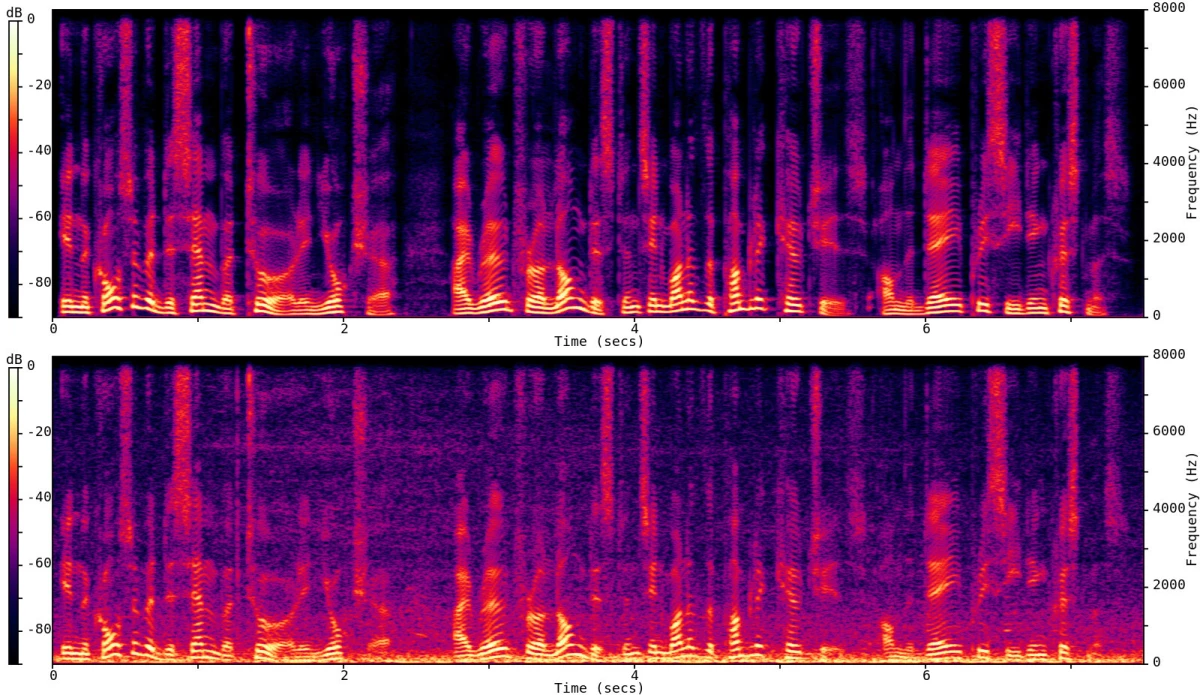\n\nThe spectrograms above show the frequency content of an audio clip. The horizontal axis is time, the vertical axis is frequency, and the color represents the amount of energy at a particular time, for a particular frequency, using a log scale.\n\nFrom the noisy STFT, many algorithms try to estimate the clean magnitude of each frequency while retaining the phase — which is much harder to estimate — from the noisy signal. For now, let's assume we have a magic model (an oracle) that's able to do a perfect mapping from noisy spectral magnitudes to clean. This is why we started from a synthetic example, so we can compute the oracle output. Based on oracle magnitudes but using the noisy phase, we can reconstruct the speech signal:\n\nCertainly not bad, but also far from perfect. The noise is still audible as a form of roughness in the speech. This is due to the error in the phase, which we took from the noisy signal. While the ear is essentially insensitive to the absolute phase, what we perceive here is the inconsistency of the phase across frames. In other words, the way in which the phase changes over time still does matter.\n\nAnother issue for real-time, power-constrained operation is the number of frequency bins whose amplitudes we need to estimate. Assuming we use 20-millisecond windows, the STFT bins will be spaced 50 Hz apart. If we want to enhance all frequencies up to 20 kHz (the upper limit of human hearing), then our neural network will have to estimate 400 amplitudes, which is very computationally expensive.\n\nWhere do we go from here? If we want to improve quality, then we could also estimate phase. This is the no-compromise route taken by PoCoNet, which can get around the added complexity because it’s optimized to run on a GPU. For real-time applications on power-constrained devices, however, we can't realistically expect to have a very good phase estimator.\n\n#### **A perceptually relevant representation**\n\nIf we want good speech quality, and we want our algorithm to run in real time on a CPU without instantly draining the battery, then we need to find a way to simplify the problem. We can do that by making the following assumptions:\n\n1. the general shape of the speech spectrum (a.k.a. the spectral envelope) is smooth; and \n2. we perceive it with a nonlinear frequency resolution, corresponding to the human ear’s auditory filters (a.k.a. critical bands)\n\nIn other words, (1) the speech spectrum tends not to have sharp discontinuities, and (2) the human auditory system perceives low frequencies with higher resolution than high frequencies.\n\nWe can follow both of those assumptions by representing the speech spectrum using bands spaced according to equivalent rectangular bandwidth (ERB). ERB-spaced bands divide the spectrum into bands of increasing width, capturing coarser spectral information as frequency increases, much the way the human auditory system does.\n\nBecause multiple STFT bins are assigned to each band, the spectral representation is smoother: any discontinuity in frequency is averaged out.\n\nNonlinearly spaced bands make our model much simpler. Instead of 400 frequency bins, we need only 34 bands. In practice, we model these bands as overlapping filters, which are most responsive to the frequencies at the centers of the bands (the tips of the triangles below) and decreasingly responsive to frequencies farther from the center (the sides of the triangles; note the 50% overlap between bands):\n\n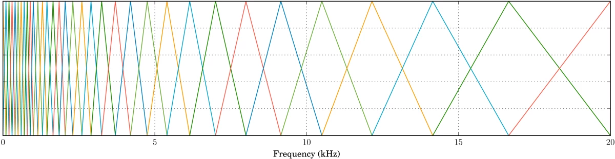\n\nFor each of the bands above, we compute a gain between 0 and 1; then, all we need to do is interpolate those band gains and we're done. Now, let's listen to how this would sound — still using the oracle for band magnitudes:\n\nOur complexity went down, but so did the quality. The roughness we noticed previously is now even more obvious and sounds a bit like heavy distortion. It's not that surprising, since we are still changing only the magnitude spectrum, but with only 34 degrees of freedom rather than 400.\n\nSo what are we missing here? The missing piece is that the ear doesn't only perceive the spectral envelope of the signal; it also perceives whether the signal is made of tones (voiced sounds), noise (unvoiced sounds), or a mix of the two. Vowels are mostly composed of tones (harmonics) at multiples of a fundamental frequency (the pitch), whereas many consonants (such as the /s/ phoneme) are mostly noise-like. \n\nOur enhanced speech sounds rough because the tonal vowels contain more noise than they should. To enhance our tones, we can use a time-domain technique called comb filtering. Comb filtering is often an undesired effect in which room reverberation boosts or attenuates frequencies at regular intervals. But by carefully tuning our comb filter to the pitch of the voice we're trying to enhance, we can keep all the tones and remove most of the noise. Below is an example of the frequency response of the comb filter for a pitch of 200 Hz.\n\n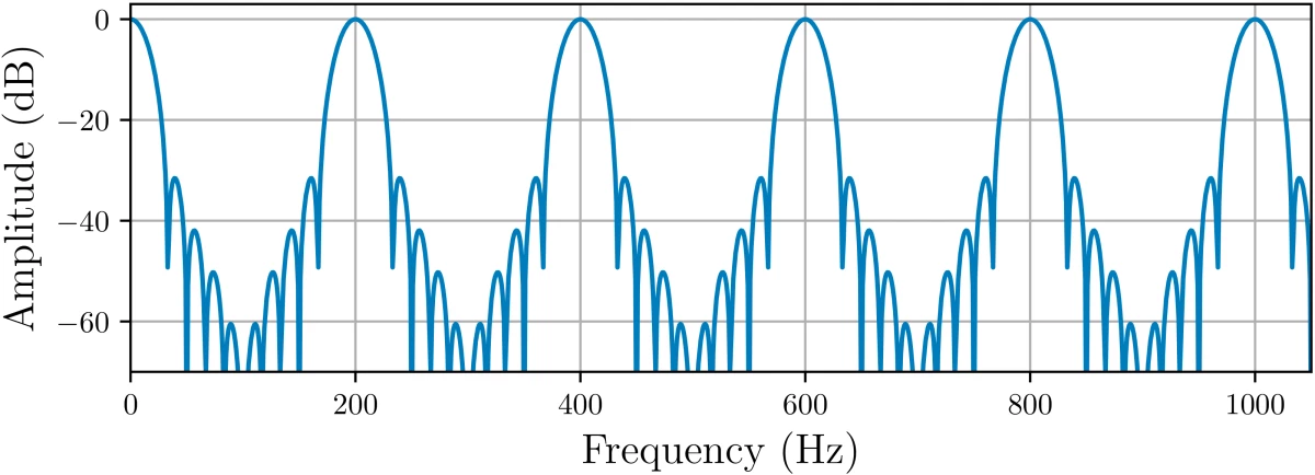\n\nThe pitch is the period at which a periodic signal (nearly) repeats itself. Pitch estimation is a hard problem, especially in the noisy conditions we have here. To estimate the pitch, we try to match a signal with past versions of itself, finding the period T that maximizes the correlation between x(n) and x(n-T). We then use dynamic programming (the Viterbi algorithm) to find a pitch trajectory that is consistent (e.g. no large jumps) over time.\n\nSince we often want to retain at least some of the noise, we can simply do a mix between the noisy audio and the comb-filtered audio to get exactly the tone/noise ratio we want. By doing the mixing in the frequency domain, we can control that mix on a band-by-band basis, even though the comb filter is computed in the time domain. The exact ratios (or filtering strengths) to use for the mixing can be adjusted in such a way that the ratio of tones to noise in the output is about the same as it was in the clean speech. This is what our oracle (using the optimal strengths) now sounds like with comb filtering:\n\nThere’s still a little roughness, but our quality is already better than that of our spectral-magnitude oracle, despite using far fewer parameters. It now seems that we're as close to the original properties of the speech as we could get with our model. So what else can we do to further improve quality? The answer is simple: we cheat! \n\nTo be more specific, we can cheat the human auditory system a bit by further attenuating the frequency bands that are still too noisy. Our speech will deviate slightly from the correct spectral envelope, but the ear will not notice that too much. It will just notice the noise less. This kind of post-filtering has been used in speech codecs since the 1980s but (as far as we know) not in speech enhancement systems. Adding the post-filter to our oracle gives us the following:\n\nWe're now quite close to the perfect clean speech. At this point, our limiting factor will most certainly be the DNN model and not the representation we use. The good thing is that our DNN has to estimate only 34 band gains (between 0 and 1) and 34 comb-filtering strengths (also between 0 and 1). This is much easier than estimating 400 magnitudes/gains — and possibly also 400 phases.\n\n#### **Adding a DNN**\n\nSo far, we’ve assumed a perfect model for predicting band gains (the oracle). In practice, we need to use a DNN. But all the work we did in the previous section was meant to make the DNN design as boring as possible.\n\nSince we replaced our initial 400 frequency bins with just 34 bands, there's no reason to use convolutional layers across frequency. Instead, we just go with convolutional layers across time and — most importantly — recurrent layers that provide longer-term memory to the system. We found that simple gated recurrent units (GRUs) work well, but long-short-term-memory networks (LSTMs) would probably have worked as well.\n\nIn our **DNN model, f** is an input feature vector that contains all the band-based spectral information we need. The outputs are the band gains ĝb and the comb-filtering strengths r̂b. Now all we need to do is train our network using hours of clean speech to which we add various levels of noise and reverberation. Since we have the clean speech, we can compute the optimal (oracle) gains and filtering strengths and use them as training targets. Our complete system using the trained DNN sounds like this:\n\n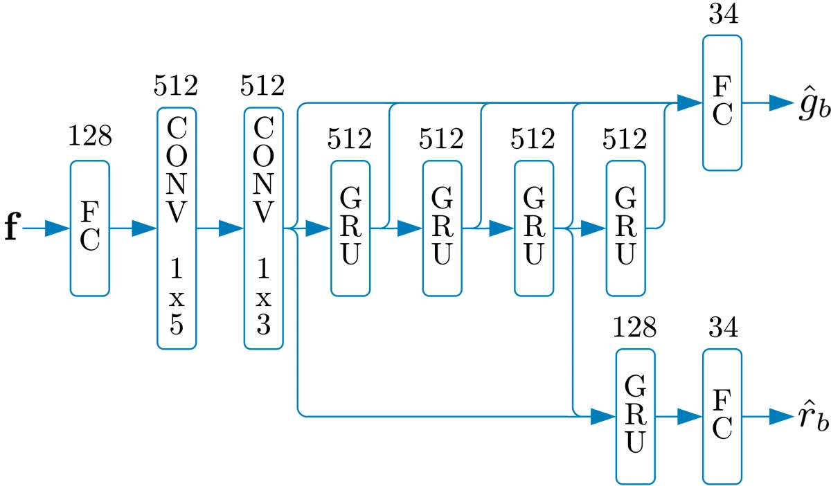\n\nDNN model\n\nObviously, it does not sound as good as the last oracle — no enhancement DNN is perfect — but it's still a big improvement over the noisy input speech. Our Interspeech 2020 Deep Noise Suppression Challenge [samples page](https://www.amazon.science/interspeech-2020-deep-noise-suppression-audio-samples) provides some examples of how PercepNet performs in real conditions.\n\n#### **Using it in real time**\n\nThe DNN model above contains about eight million weights. For each new window, we use each weight exactly once, which means eight million multiply-add operations per window. With 20-millisecond windows and 50% overlap, we have 100 windows per second of speech, so 800 million multiply-add operations per second. \n\nThankfully, DNNs tend to be quite robust to small perturbations, so we can quantize all our weights to just eight bits with a negligible effect on perceived audio quality. Thanks to SIMD instructions on modern CPUs, this makes it possible to run our network really efficiently. On a modern laptop CPU, it takes less than 5% of one core to run PercepNet in real time.\n\nTo be useful in real-time communications applications, PercepNet should not add too much delay. The seemingly arbitrary choice of 20-millisecond windows with 50% overlap means that it consumes audio 10 milliseconds at a time. This is good because most audio codecs (including Opus, which is used in WebRTC) encode audio in 20-millisecond packets. So we can run the algorithm exactly twice per packet without the PercepNet block size causing an increase in delay. \n\nThere are, of course, some delays we cannot avoid. The overlap between windows means that the STFT itself requires 10 milliseconds for reconstruction. On top of that, we typically allow the DNN to look two windows (20 millseconds) into the future, so it can make better decisions. This gives us a total of 30 milliseconds extra delay from the algorithm, which is acceptable in most scenarios.\n\nIf you would like to know more about the details of PercepNet, you can [read our Interspeech 2020 paper](https://www.amazon.science/publications/a-perceptually-motivated-approach-for-low-complexity-real-time-enhancement-of-fullband-speech). The idea behind PercepNet is quite versatile and could be applied to other problems, including acoustic echo control and beamforming post-filtering. In future posts, we will see how we can make PercepNet very efficient on CPUs and even how to run it as Web Assembly (WASM) code inside web browsers for WebRTC-based applications.\n\n","render":"<p>PercepNet is one of the core technologies of Amazon Chime’s <a href=\"https://docs.aws.amazon.com/chime/latest/ug/voice-focus.html\" target=\"_blank\">Voice Focus</a> feature. It is designed to suppress noise and reverberation in the speech signal, in real time, without using too many CPU cycles. This makes it usable in cellphones and other power-constrained devices.</p>\n<p>At Interspeech 2020, PercepNet f<a href=\"https://www.amazon.science/blog/amazon-team-takes-first-place-in-interspeech-2020-deep-noise-suppression-challenge\" target=\"_blank\">inished second in its category</a> (real-time processing) in the Deep Noise Suppression Challenge, despite using only 4% of a CPU core, while another Amazon Chime algorithm, PoCoNet, finished first in the offline-processing category. In this post, we’ll look into the principles that make PercepNet work. For more details, you can also refer to our <a href=\"https://www.amazon.science/publications/a-perceptually-motivated-approach-for-low-complexity-real-time-enhancement-of-fullband-speech\" target=\"_blank\">Interspeech paper</a>.</p>\n<p>Despite operating in real time, with low complexity, PercepNet can still provide state-of-the-art speech enhancement. Like most recent speech enhancement algorithms, PercepNet uses deep learning, but it applies it in a different way. Rather than have a deep neural network (DNN) do all the work, PercepNet tries to have it do as little work as possible.</p>\n<h4><a id=\"Speech_enhancement_and_STFT_6\"></a><strong>Speech enhancement and STFT</strong></h4>\n<p>Before getting into any deep learning, let’s look at the job we’ll be asking our machine learning model to perform. Let’s consider a simple synthetic example. We start from the clean speech sample below:</p>\n<p>We then add some non-stationary car noise on top of it:</p>\n<p>The goal here is to take the noisy audio and make it sound as good as possible — ideally, close to the original clean audio. The standard way to represent the problem — both pre-deep learning and post-deep learning — is to use the <a href=\"https://en.wikipedia.org/wiki/Short-time_Fourier_transform\" target=\"_blank\">short-time Fourier transform </a>(STFT).</p>\n<p>That means chopping up the signal into overlapping windows and computing the frequency content for each window. For each window of N samples (N discrete measurements of the signal amplitude), we obtain N/2 spectral magnitudes, along with their associated phases. We will refer to each output point as a frequency bin. Let’s see what the magnitude of the STFT looks like for our clean signal (top) and noisy signal (bottom).</p>\n<p><img src=\"https://dev-media.amazoncloud.cn/c5cb84fc7d5847779b3385d5fb74bc91_image.png\" alt=\"image.png\" /></p>\n<p>The spectrograms above show the frequency content of an audio clip. The horizontal axis is time, the vertical axis is frequency, and the color represents the amount of energy at a particular time, for a particular frequency, using a log scale.</p>\n<p>From the noisy STFT, many algorithms try to estimate the clean magnitude of each frequency while retaining the phase — which is much harder to estimate — from the noisy signal. For now, let’s assume we have a magic model (an oracle) that’s able to do a perfect mapping from noisy spectral magnitudes to clean. This is why we started from a synthetic example, so we can compute the oracle output. Based on oracle magnitudes but using the noisy phase, we can reconstruct the speech signal:</p>\n<p>Certainly not bad, but also far from perfect. The noise is still audible as a form of roughness in the speech. This is due to the error in the phase, which we took from the noisy signal. While the ear is essentially insensitive to the absolute phase, what we perceive here is the inconsistency of the phase across frames. In other words, the way in which the phase changes over time still does matter.</p>\n<p>Another issue for real-time, power-constrained operation is the number of frequency bins whose amplitudes we need to estimate. Assuming we use 20-millisecond windows, the STFT bins will be spaced 50 Hz apart. If we want to enhance all frequencies up to 20 kHz (the upper limit of human hearing), then our neural network will have to estimate 400 amplitudes, which is very computationally expensive.</p>\n<p>Where do we go from here? If we want to improve quality, then we could also estimate phase. This is the no-compromise route taken by PoCoNet, which can get around the added complexity because it’s optimized to run on a GPU. For real-time applications on power-constrained devices, however, we can’t realistically expect to have a very good phase estimator.</p>\n<h4><a id=\"A_perceptually_relevant_representation_28\"></a><strong>A perceptually relevant representation</strong></h4>\n<p>If we want good speech quality, and we want our algorithm to run in real time on a CPU without instantly draining the battery, then we need to find a way to simplify the problem. We can do that by making the following assumptions:</p>\n<ol>\n<li>the general shape of the speech spectrum (a.k.a. the spectral envelope) is smooth; and</li>\n<li>we perceive it with a nonlinear frequency resolution, corresponding to the human ear’s auditory filters (a.k.a. critical bands)</li>\n</ol>\n<p>In other words, (1) the speech spectrum tends not to have sharp discontinuities, and (2) the human auditory system perceives low frequencies with higher resolution than high frequencies.</p>\n<p>We can follow both of those assumptions by representing the speech spectrum using bands spaced according to equivalent rectangular bandwidth (ERB). ERB-spaced bands divide the spectrum into bands of increasing width, capturing coarser spectral information as frequency increases, much the way the human auditory system does.</p>\n<p>Because multiple STFT bins are assigned to each band, the spectral representation is smoother: any discontinuity in frequency is averaged out.</p>\n<p>Nonlinearly spaced bands make our model much simpler. Instead of 400 frequency bins, we need only 34 bands. In practice, we model these bands as overlapping filters, which are most responsive to the frequencies at the centers of the bands (the tips of the triangles below) and decreasingly responsive to frequencies farther from the center (the sides of the triangles; note the 50% overlap between bands):</p>\n<p><img src=\"https://dev-media.amazoncloud.cn/2660c37409824d02ba45170d8505ec8d_image.png\" alt=\"image.png\" /></p>\n<p>For each of the bands above, we compute a gain between 0 and 1; then, all we need to do is interpolate those band gains and we’re done. Now, let’s listen to how this would sound — still using the oracle for band magnitudes:</p>\n<p>Our complexity went down, but so did the quality. The roughness we noticed previously is now even more obvious and sounds a bit like heavy distortion. It’s not that surprising, since we are still changing only the magnitude spectrum, but with only 34 degrees of freedom rather than 400.</p>\n<p>So what are we missing here? The missing piece is that the ear doesn’t only perceive the spectral envelope of the signal; it also perceives whether the signal is made of tones (voiced sounds), noise (unvoiced sounds), or a mix of the two. Vowels are mostly composed of tones (harmonics) at multiples of a fundamental frequency (the pitch), whereas many consonants (such as the /s/ phoneme) are mostly noise-like.</p>\n<p>Our enhanced speech sounds rough because the tonal vowels contain more noise than they should. To enhance our tones, we can use a time-domain technique called comb filtering. Comb filtering is often an undesired effect in which room reverberation boosts or attenuates frequencies at regular intervals. But by carefully tuning our comb filter to the pitch of the voice we’re trying to enhance, we can keep all the tones and remove most of the noise. Below is an example of the frequency response of the comb filter for a pitch of 200 Hz.</p>\n<p><img src=\"https://dev-media.amazoncloud.cn/0f373cdc94d14b1eb7d90d77c768ecf0_image.png\" alt=\"image.png\" /></p>\n<p>The pitch is the period at which a periodic signal (nearly) repeats itself. Pitch estimation is a hard problem, especially in the noisy conditions we have here. To estimate the pitch, we try to match a signal with past versions of itself, finding the period T that maximizes the correlation between x(n) and x(n-T). We then use dynamic programming (the Viterbi algorithm) to find a pitch trajectory that is consistent (e.g. no large jumps) over time.</p>\n<p>Since we often want to retain at least some of the noise, we can simply do a mix between the noisy audio and the comb-filtered audio to get exactly the tone/noise ratio we want. By doing the mixing in the frequency domain, we can control that mix on a band-by-band basis, even though the comb filter is computed in the time domain. The exact ratios (or filtering strengths) to use for the mixing can be adjusted in such a way that the ratio of tones to noise in the output is about the same as it was in the clean speech. This is what our oracle (using the optimal strengths) now sounds like with comb filtering:</p>\n<p>There’s still a little roughness, but our quality is already better than that of our spectral-magnitude oracle, despite using far fewer parameters. It now seems that we’re as close to the original properties of the speech as we could get with our model. So what else can we do to further improve quality? The answer is simple: we cheat!</p>\n<p>To be more specific, we can cheat the human auditory system a bit by further attenuating the frequency bands that are still too noisy. Our speech will deviate slightly from the correct spectral envelope, but the ear will not notice that too much. It will just notice the noise less. This kind of post-filtering has been used in speech codecs since the 1980s but (as far as we know) not in speech enhancement systems. Adding the post-filter to our oracle gives us the following:</p>\n<p>We’re now quite close to the perfect clean speech. At this point, our limiting factor will most certainly be the DNN model and not the representation we use. The good thing is that our DNN has to estimate only 34 band gains (between 0 and 1) and 34 comb-filtering strengths (also between 0 and 1). This is much easier than estimating 400 magnitudes/gains — and possibly also 400 phases.</p>\n<h4><a id=\"Adding_a_DNN_65\"></a><strong>Adding a DNN</strong></h4>\n<p>So far, we’ve assumed a perfect model for predicting band gains (the oracle). In practice, we need to use a DNN. But all the work we did in the previous section was meant to make the DNN design as boring as possible.</p>\n<p>Since we replaced our initial 400 frequency bins with just 34 bands, there’s no reason to use convolutional layers across frequency. Instead, we just go with convolutional layers across time and — most importantly — recurrent layers that provide longer-term memory to the system. We found that simple gated recurrent units (GRUs) work well, but long-short-term-memory networks (LSTMs) would probably have worked as well.</p>\n<p>In our <strong>DNN model, f</strong> is an input feature vector that contains all the band-based spectral information we need. The outputs are the band gains ĝb and the comb-filtering strengths r̂b. Now all we need to do is train our network using hours of clean speech to which we add various levels of noise and reverberation. Since we have the clean speech, we can compute the optimal (oracle) gains and filtering strengths and use them as training targets. Our complete system using the trained DNN sounds like this:</p>\n<p><img src=\"https://dev-media.amazoncloud.cn/108e389f31e0491a98b25d113135ac9a_image.png\" alt=\"image.png\" /></p>\n<p>DNN model</p>\n<p>Obviously, it does not sound as good as the last oracle — no enhancement DNN is perfect — but it’s still a big improvement over the noisy input speech. Our Interspeech 2020 Deep Noise Suppression Challenge <a href=\"https://www.amazon.science/interspeech-2020-deep-noise-suppression-audio-samples\" target=\"_blank\">samples page</a> provides some examples of how PercepNet performs in real conditions.</p>\n<h4><a id=\"Using_it_in_real_time_79\"></a><strong>Using it in real time</strong></h4>\n<p>The DNN model above contains about eight million weights. For each new window, we use each weight exactly once, which means eight million multiply-add operations per window. With 20-millisecond windows and 50% overlap, we have 100 windows per second of speech, so 800 million multiply-add operations per second.</p>\n<p>Thankfully, DNNs tend to be quite robust to small perturbations, so we can quantize all our weights to just eight bits with a negligible effect on perceived audio quality. Thanks to SIMD instructions on modern CPUs, this makes it possible to run our network really efficiently. On a modern laptop CPU, it takes less than 5% of one core to run PercepNet in real time.</p>\n<p>To be useful in real-time communications applications, PercepNet should not add too much delay. The seemingly arbitrary choice of 20-millisecond windows with 50% overlap means that it consumes audio 10 milliseconds at a time. This is good because most audio codecs (including Opus, which is used in WebRTC) encode audio in 20-millisecond packets. So we can run the algorithm exactly twice per packet without the PercepNet block size causing an increase in delay.</p>\n<p>There are, of course, some delays we cannot avoid. The overlap between windows means that the STFT itself requires 10 milliseconds for reconstruction. On top of that, we typically allow the DNN to look two windows (20 millseconds) into the future, so it can make better decisions. This gives us a total of 30 milliseconds extra delay from the algorithm, which is acceptable in most scenarios.</p>\n<p>If you would like to know more about the details of PercepNet, you can <a href=\"https://www.amazon.science/publications/a-perceptually-motivated-approach-for-low-complexity-real-time-enhancement-of-fullband-speech\" target=\"_blank\">read our Interspeech 2020 paper</a>. The idea behind PercepNet is quite versatile and could be applied to other problems, including acoustic echo control and beamforming post-filtering. In future posts, we will see how we can make PercepNet very efficient on CPUs and even how to run it as Web Assembly (WASM) code inside web browsers for WebRTC-based applications.</p>\n"}